Example Variables(Open Data):

The Fennema-Sherman Mathematics Attitude Scales (FSMAS) are among the most popular instruments used in studies of attitudes toward mathematics. FSMAS contains 36 items. Also, scales of FSMAS have Confidence, Effectance Motivation, and Anxiety. The sample includes 425 teachers who answered all 36 items. In addition, other characteristics of teachers, such as their age, are included in the data.
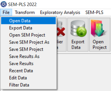
You can select your data as follows:
1-File
2-Open data
(See Open Data)

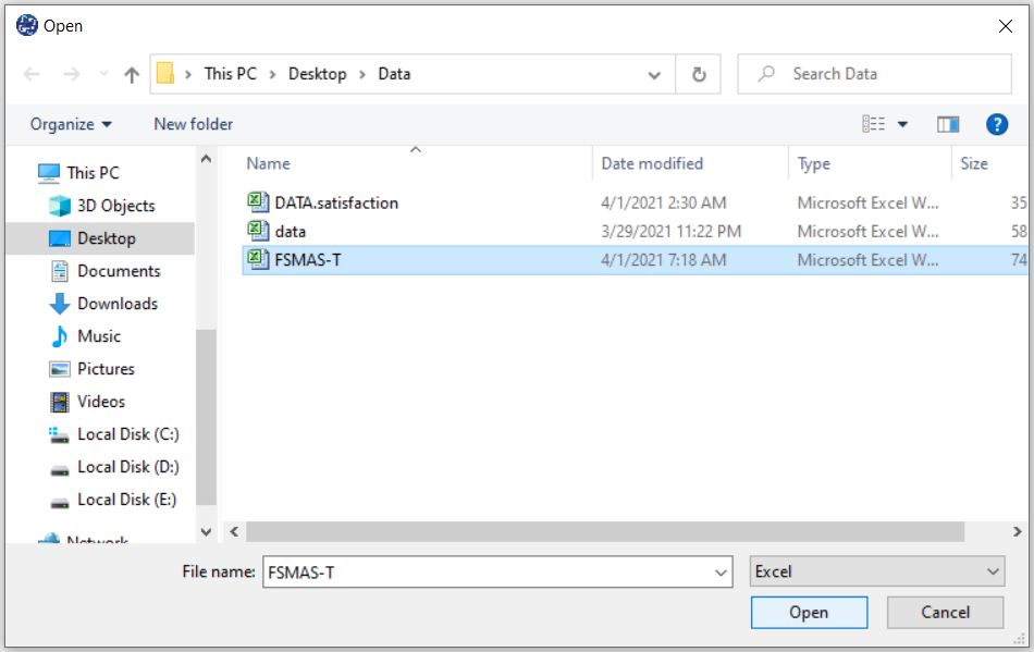
The data is stored under the name FSMAS-T(You can download this data from here ).
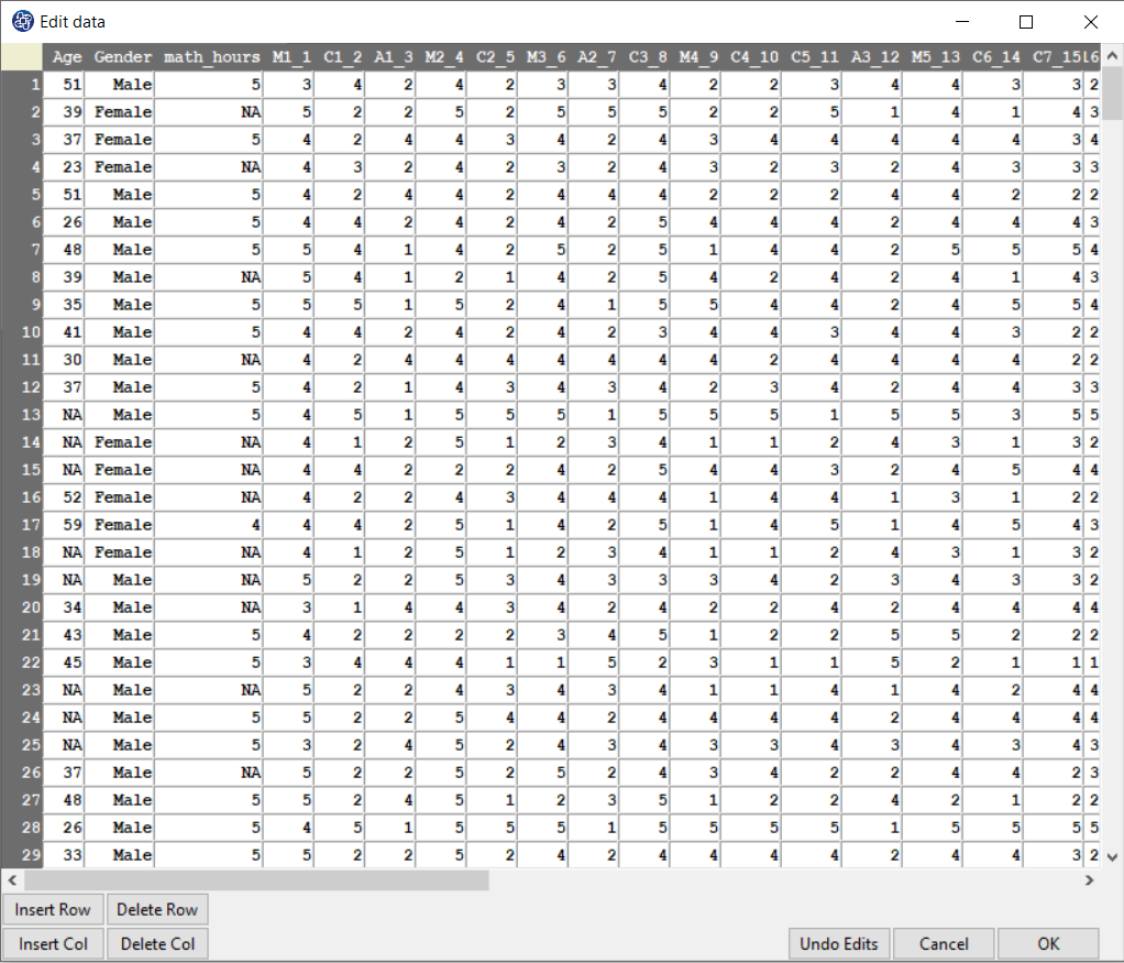
You can edit the imported data via the following path:
1-File
2-Edit Data
(See Edit Data)

Path of Path Analysis:

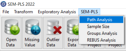
You can perform Path Analysis by the following path or Path Analysis button:
1-SEM-PLS
2- Path Analysis

A. Path Analysis:

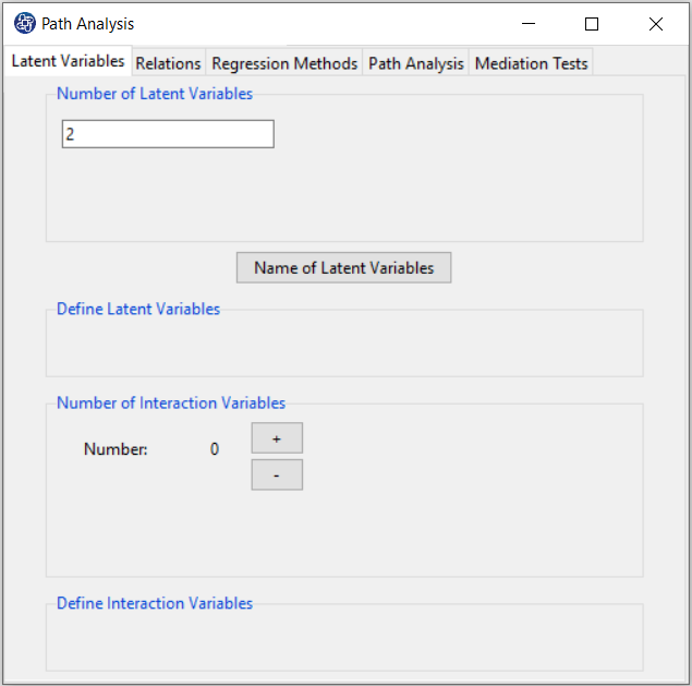
Path Analysis window includes five tabs, Latent Variables, Relations, Regression Methods, Path Analysis, and Mediation Tests.
To fit the model, you must perform the following steps:

In Latent Variables tab:
1- Determine the number of latent variables.
2- Specify the name of each latent variable.
3-Define latent variables.
3.1- If the model has interaction variables, you can first determine the number of interaction variables and then specify them.

In Relation tab:
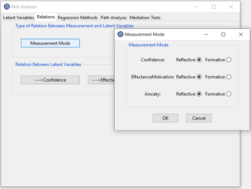
4- Specify the type of Outer model(type of relation between measurement variables and latent variable)
5- Specify Inner models(relation between latent variables)

In the Regression Methods tab:
6- You must specify the type of regression method for each Inner model.

In the Path Analysis tab:
7- Finally, you can run the model, view and save the results.

In the Mediation Tests tab:
7.1- If the model has an indirect relationship, you can test the significance of the effect of mediating variables.

D. Model without Interaction Variable:

D1. Step1:

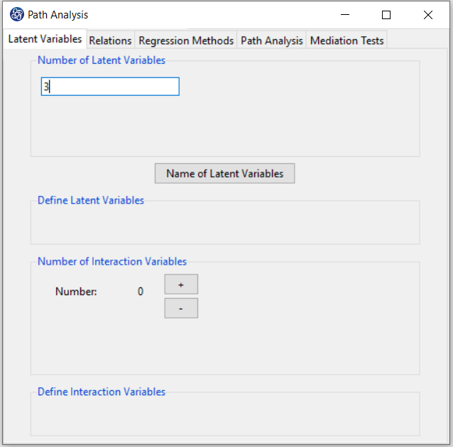
First, you must determine the number of latent variables in the Number of Latent Variables.
For example, you can set the number of latent variables to 3.

D2. Step2:

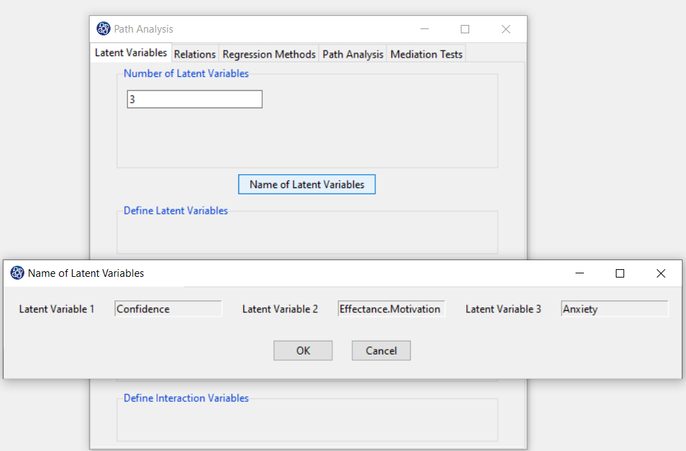
By clicking on the “Name of Latent Variables” button, you can specify the names of the latent variables.
For Example, After clicking on the “Name of Latent Variables” button, in front of the names Latent Variable 1, Latent Variable 2, and Latent Variable 3, we type the names of Confidence, Effectance.Motivation, and Anxiety.
After clicking on the "OK" button in “Name of Latent Variables” window, separate buttons with the name of latent variables are created in the “Define Latent Variables” panel.

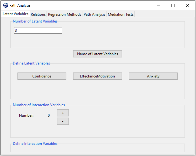
D3. Step3:

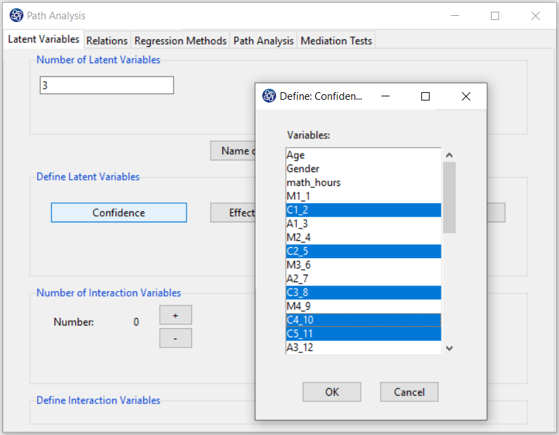
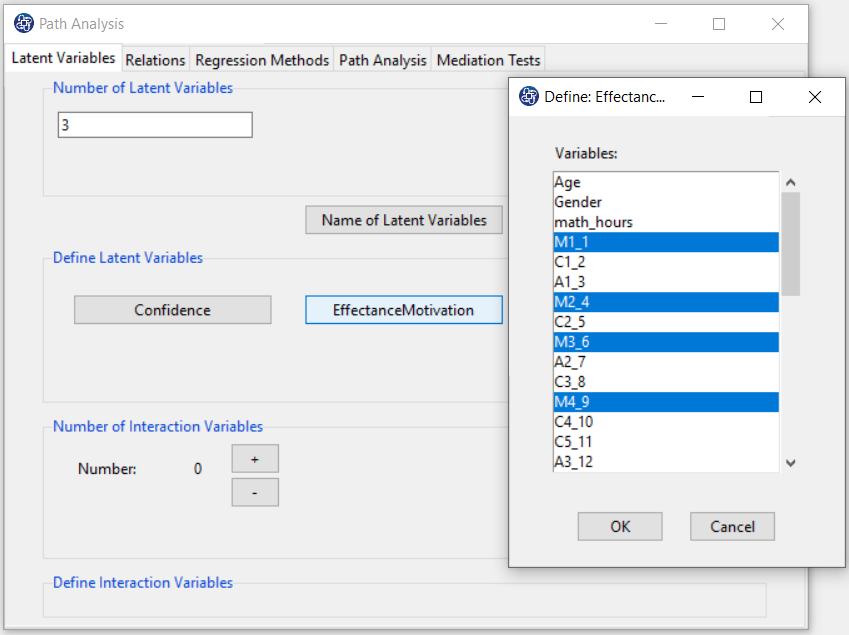
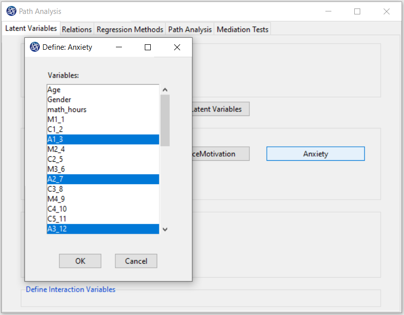
In Define Latent Variables, you must click on the name of each of the latent variables. Then select the corresponding measurement variables for each latent variable.
For example, you are clicking on any of the variables of Confidence, Effectance.Motivation, and Anxiety opens a window for selecting variables. Items starting with the letters C, M, and A are related to Confidence, Effectance Motivation, and Anxiety, respectively.

D4. Relations tab:

This tab has two panels, “Type of Relation Between Measurement and Latent Variable” and “Relation Between Latent Variables”, which are used to perform steps 4 and 5, respectively.

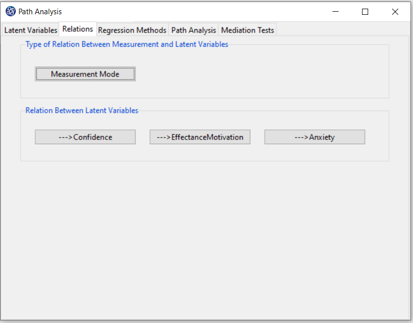
D5. Step4:

This tab has two panels, “Type of Relation Between Measurement and Latent Variable” and “Relation Between Latent Variables”, which are used to perform steps 4 and 5, respectively.

D6. Step5:

This tab has two panels, “Type of Relation Between Measurement and Latent Variable” and “Relation Between Latent Variables”, which are used to perform steps 4 and 5, respectively.

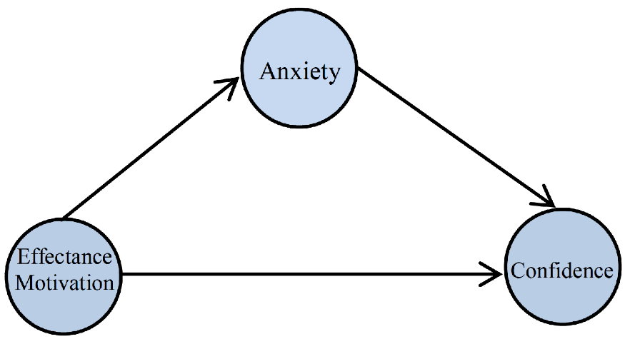
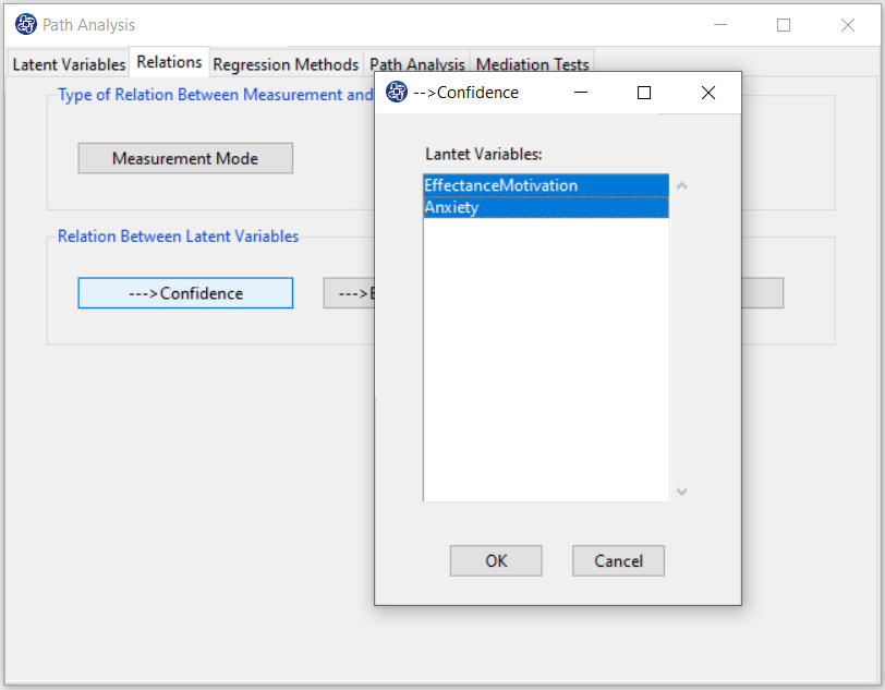
--->Confidence: You have to click on the “--->Confidence” button to select the variables that affect it, namely EffectanceMotivation, and Anxiety.

--->EffectanceMotivation: For this model, you do not need to click on this variable because no variable will affect this variable.

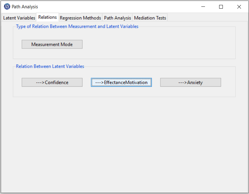
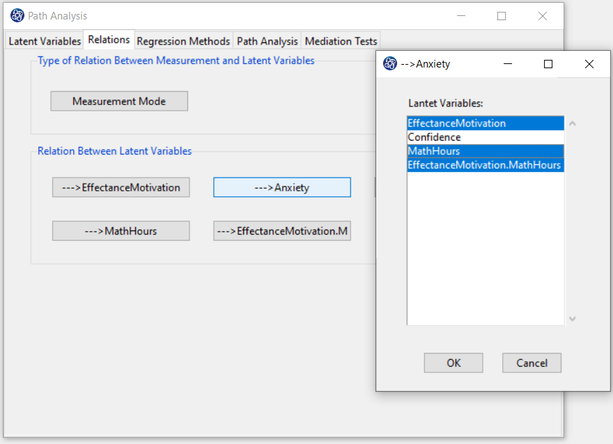
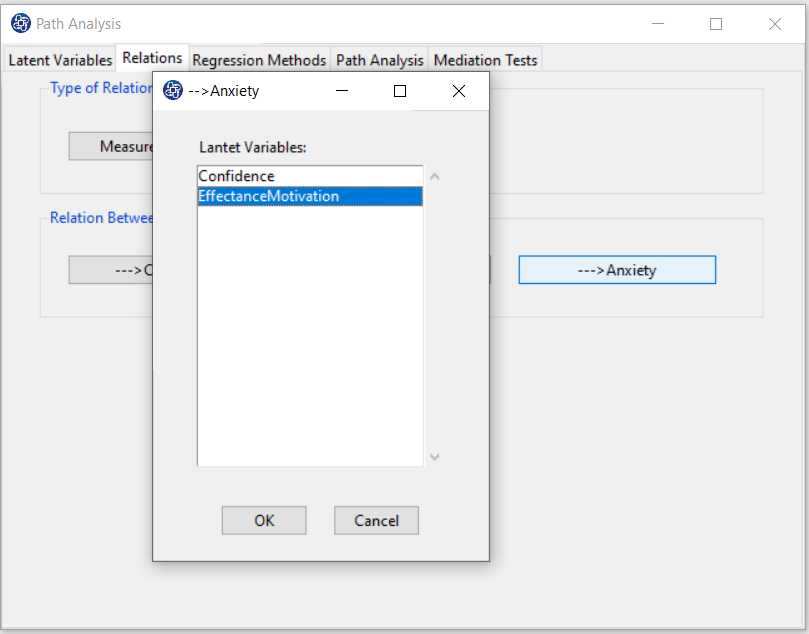
--->Anxiety: You have to click on the “--->Anxiety” button to select the variable that affects it, namely EffectanceMotivation.
Thus, you will have the following two regression models to fit this conceptual model to the data:





Which the software symbolically displays as follows:

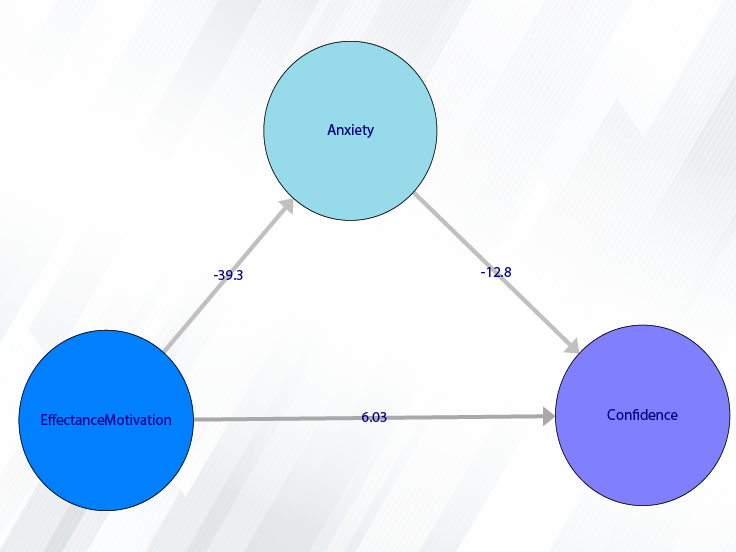
EffectanceMotivation + Anxiety---> Confidence
EffectanceMotivation ---> Anxiety

D7. Step6:

In the “Regression Methods” tab, for each of the inner models, the type of regression method can be selected.
In this tab, In front of each of the models is the “Regression Method” button, which clicking on it opens the regression method window.
This window contains seven panels.
1- “Regression Method” panel includes regression methods that should be determined based on the type of dependent variable.
2- Bootstrap Options: If you choose one of OLS(bootstrap), GLM(Bootstrap), Multinomial(Bootstrap), and MANOVA(Bootstrap), this panel controls the bootstrap method features used in that regression method (See Regression-OLS, Regression-GLM, Regression-Multinomial, Regression-MANOVA).

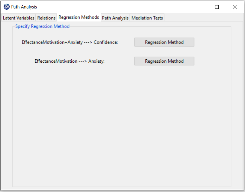
*Replication: Number of Replication(B in equations)
*Set Seed: An arbitrary number will keep the Bootstrap results fixed by holding it fixed.
3-GLM Option: See Regression-GLM
4- Ridge Option: See Regression-Ridge
5-Multinomial Option: See Regression-Multinomial
6- SUR Option: See Regression-SUR
7- MANOVA Option: See Regression-MANOVA
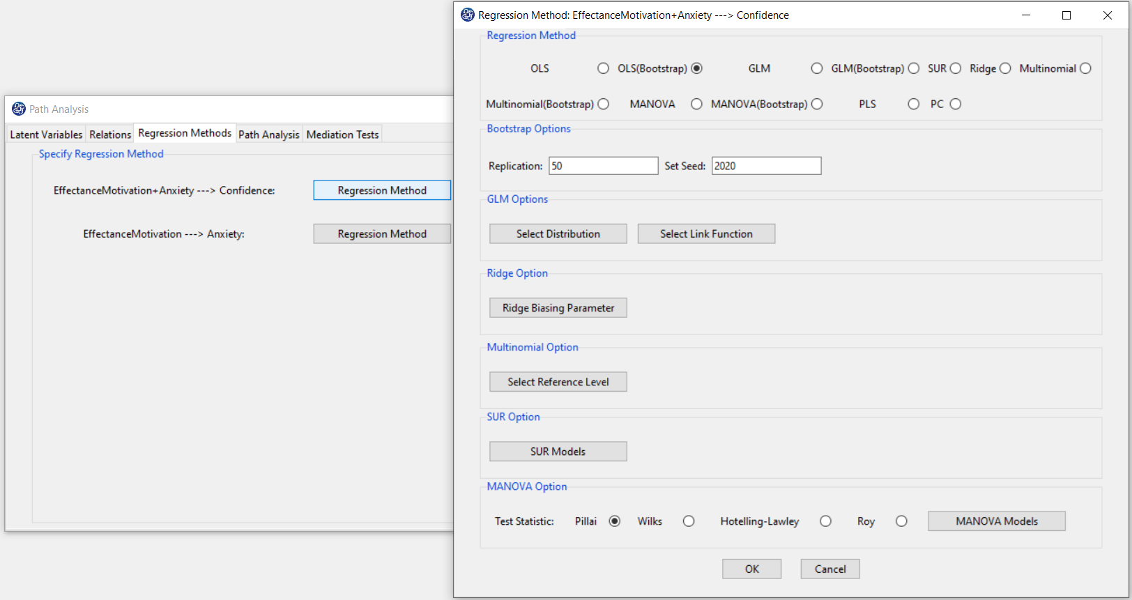
The default regression method is determined based on the type of dependent variable. For example, if the dependent variable is continuous, the default is OLS(Bootstrap) regression method.
For example, the regression method of inner model
EffectanceMotivation + Anxiety---> Confidence
can be one of the methods of OLS, OLS(Bootstrap), GLM, Ridge, PLS, and PC.

D8. Step7:

In the “Path Analysis” tab, you can view and save the fitted model results. You can plot, edit and save the model path diagram.
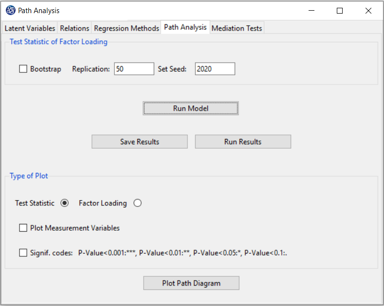
In “Test Statistic of Factor Loading”, if you want to test the effect of the measurement variables, you can activate the “Bootstrap” option. The Bootstrap test is performed with the following features:
*Replication: Number of Replication (B in equations)
*Set Seed: It is an arbitrary number that will keep the Bootstrap results fixed by holding it fixed.

D8.1. Run Model:

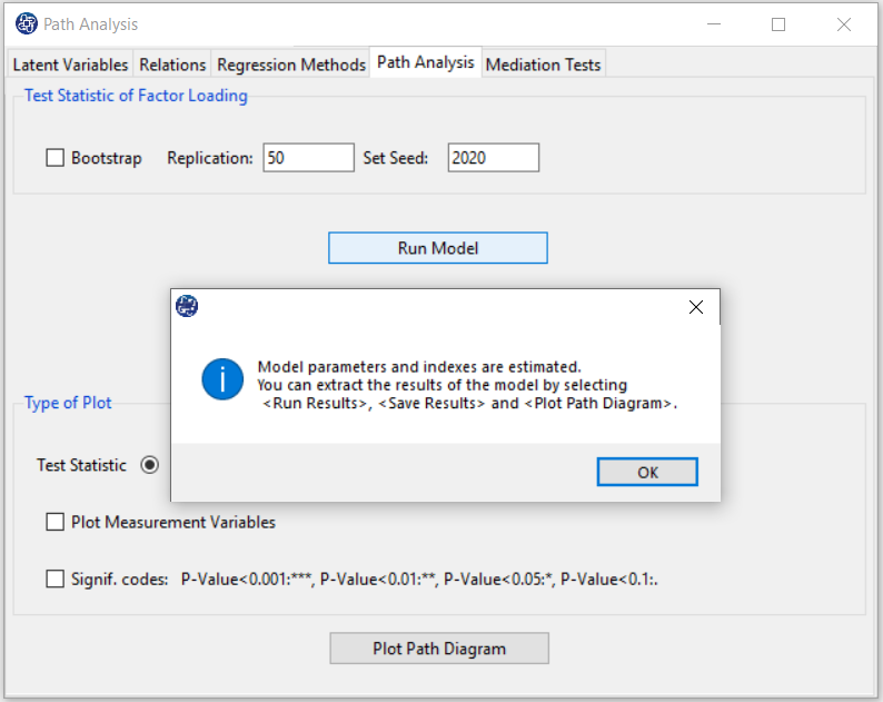
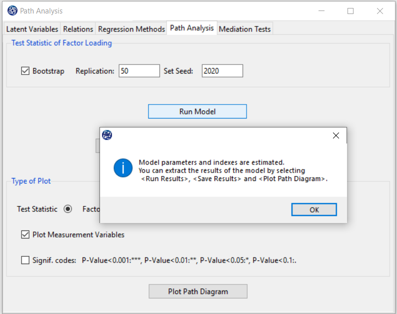
By clicking this button, you can fit the SEM model. If the model fits without problems, this message appears:
“Model parameters and indexes are estimated.
You can extract the results of the model by selecting < Run Results>, < Save Results>, and < Plot Path Diagram>.”

D8.2. Run Result:

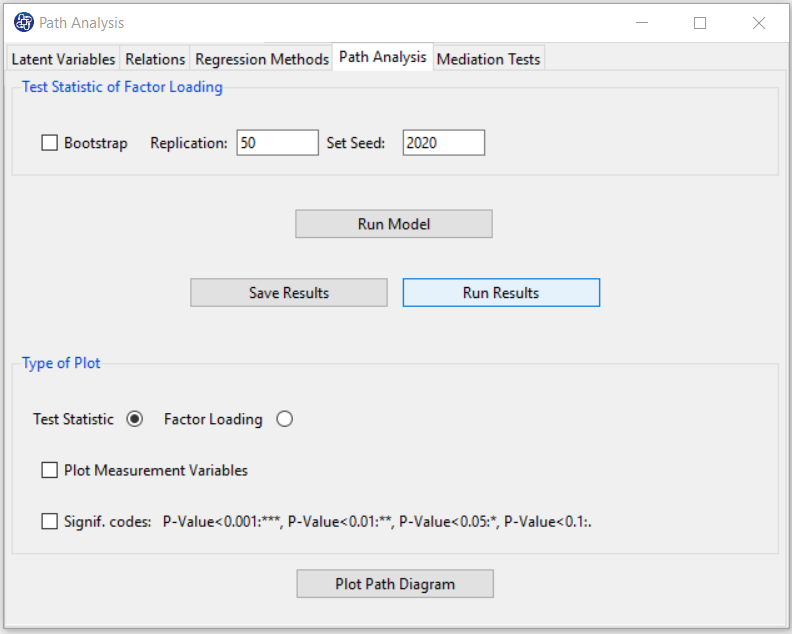
After clicking on the “Run Results” button, you can see the model fit results in the main software window.

D8.2.1. Unidimensionality:

This table shows information about the validation indexes of outer models. In this table,
*Mode: Type of outer model(A: Reflective and B:Formative)
(See Introduction to SEM-PLS: A. The Outer Model (The Measurement Model))
*MVs: Number of the measurement variable
*C.alpha: Cronbach’s Alpha (See Introduction to SEM-PLS: E.1.1. Reliability)
*DG.rho: Dillon- Goldstein’s Rho (Composite Reliability) (See Introduction to SEM-PLS: E.1.1. Reliability)
*Eigenvalue: A validation criterion is eigen of the Correlation matrix of each set of indicators. The use of this metric is based on the importance of the first eigenvalue (eig.1st). If a block is unidimensional, then the first eigenvalue (eig.1st) should be “much more” larger than 1 whereas the second eigenvalue(eig.2nd) should be smaller than 1.

D8.2.2. Outer models:

You can see the results of the outer model in this section. These results include the following:
*name: Name of measurement variables
*block: Name of latent variables
*weight: The simple regression coefficient between the measurement variable and the latent variable. (See Introduction to SEM-PLS: A. The Outer Model (The Measurement Model) )
*loading: Loading Value (See Introduction to SEM-PLS: C.3. Loadings calculation )
* communality: Communality Index (See Introduction to SEM-PLS: E.1.2. Convergent Validity )
* redundancy: Redundancy index (See Introduction to SEM-PLS:E.2.Validation of formative outer models )

D8.2.3. Cross Loadings:

You can see the Cross Loading index for any measurement variable. In this table:
*name: Name of measurement variables
*block: Name of latent variables
*Column named as latent variables: the value of Cross Loading of the measurement and latent variable. (See Introduction to SEM-PLS: C.3. Loadings calculation)

D8.2.4. Summary Inner:

A summary of the results of the latent variables is given in the Summary Inner table.
In this table,
*Type: Specifies the type of variable. Exogenous(Endogenous) mean that latent variable is a independent variable(dependent variable).
*Block_Communality:This index is equal to the average of the Communalities related to the latent variable. ( See Introduction to SEM-PLS: E.1.2. Convergent Validity)
* Mean_Redundancy: This index is equal to the average of the Redundancy related to the latent variable. (See Introduction to SEM-PLS:E.2.Validation of formative outer models)
*AVE: Average Variance Extracted (See Introduction to SEM-PLS: E.1.2. Convergent Validity)

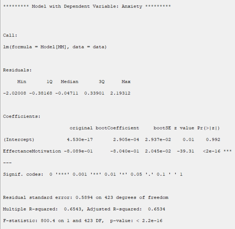
D8.2.5. Inner Models:

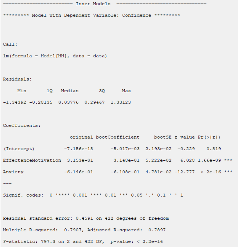
This section presents the results of the regression model. The following symbol separates each model:
“********* Model with Dependent Variable: dependent Variable *********”
For example,
“********* Model with Dependent Variable: Anxiety *********”
See details of regression methods in Regression.

D8.2.6. FORNELL-LARCKER Matrix:

This section contains the results of the FORNELL-LARCKER matrix. (See Introduction to SEM-PLS: E.1.3. Discriminant validity)

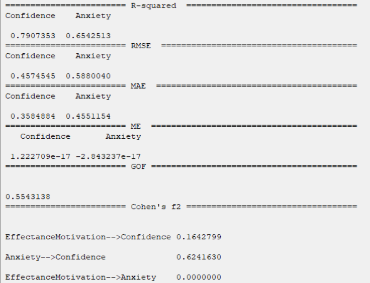
D8.2.7. Validation of Inner Models:

In this section, the validation indexes of external models are given.
In R-squared(), RMSE, MAE, ME, these indexes are separated by the name of the dependent variable. (See Introduction to SEM-PLS: E.3. Validation of inner model )

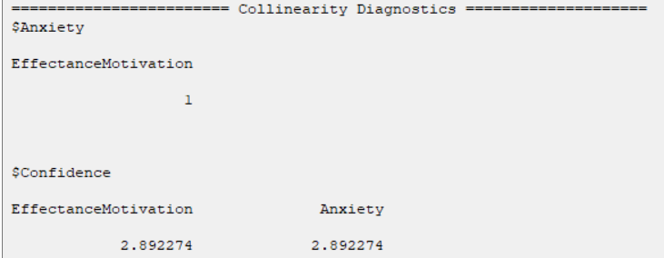
D8.2.8. Collinearity Diagnostics:

In the Collinearity Diagnostics table, the results of multicollinearity in a set of multiple regression variables are given.
For each inner model:
For each independent variable x_i, the VIF index is calculated in two steps:

STEP1:
First, we run Regression that has x_i as a function of all the other independent variables in the first equation.

STEP2:
Then, calculate the VIF factor with the following equation:
  Where   is the coefficient of determination of the regression equation in step one. Also,

A rule of decision making is that if then multicollinearity is high (a cutoff of 5 is also commonly used)

D8.2.9. Indirect Coefficients:

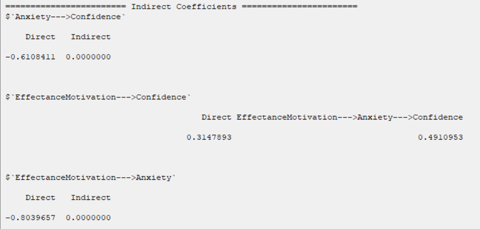
In this section, direct and indirect coefficients between hidden variables are presented. If there is no indirect relationship between the two variables, we have:
Indirect
0.0000
But, if two variables have an indirect relationship, there will be a column named their indirect relationship. For Example, in the relationship between the two variables EffectanceMotivation and Confidence, we have:
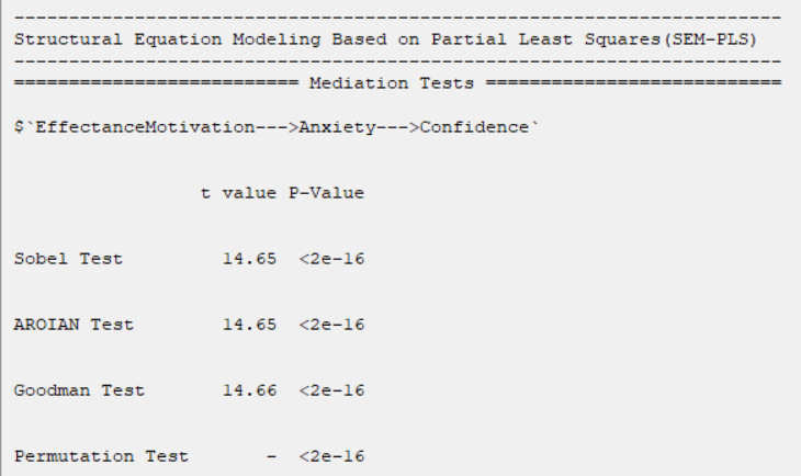
EffectanceMotivation--->Anxiety--->Confidence     0.4910953
This means that the influence coefficient of Anxiety in the relationship between these two variables is equal to 0.4910953.
(See Introduction to SEM-PLS: E.4.1. Mediation Analysis)

D8.2.10. Diagnostic Tests:

If the regression model includes diagnostic tests, it is presented in the section.

D8.3. Save Results:

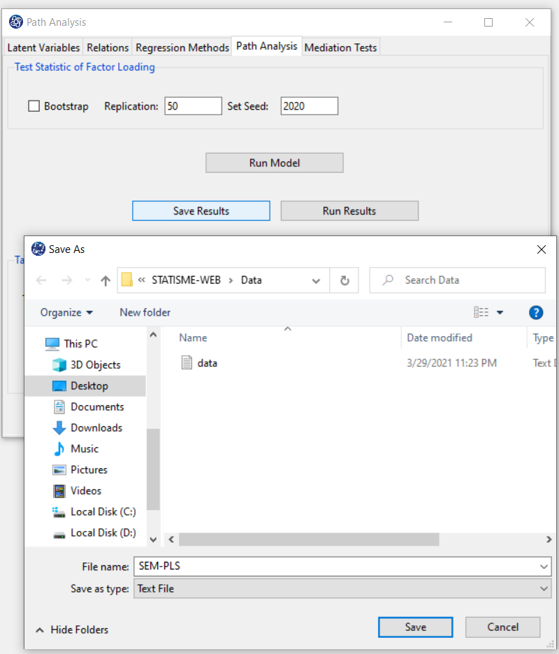
By clicking this button, you can save the SEM-PLS results. After opening the save results window, you can save the results in “text” or “Microsoft Word” format.

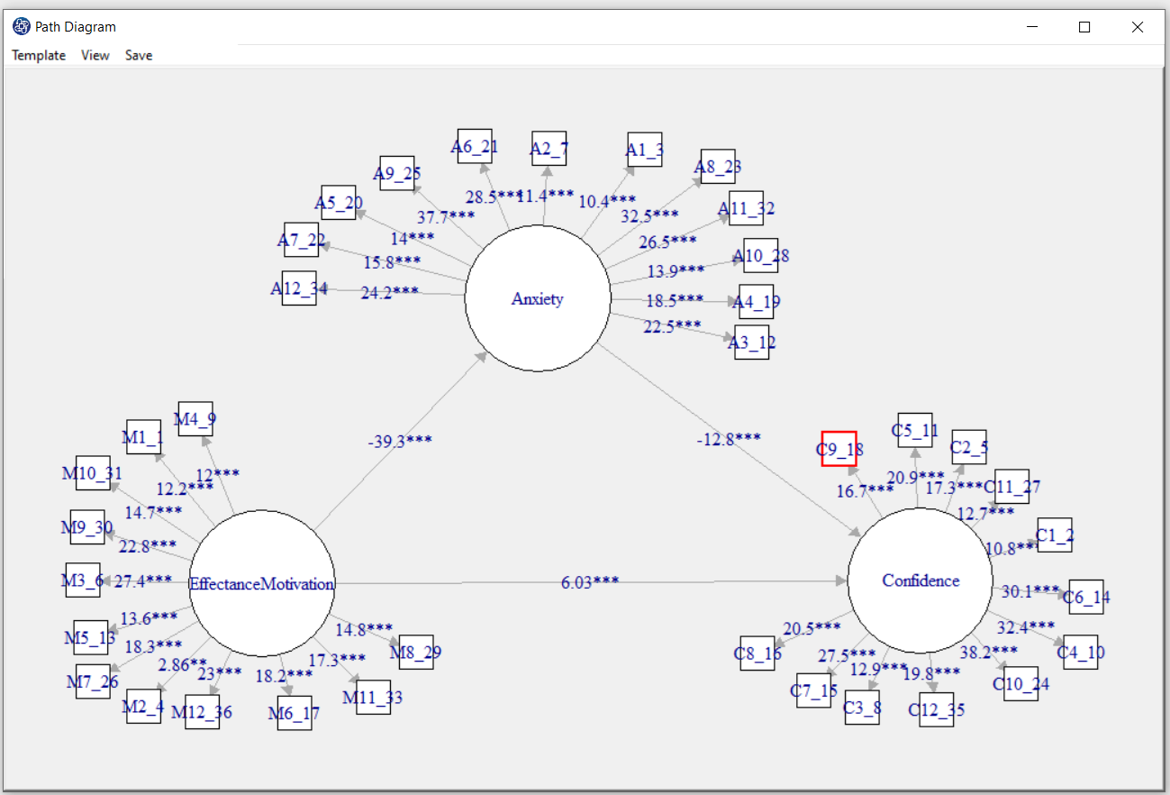
D8.4. Plot Path Diagram:

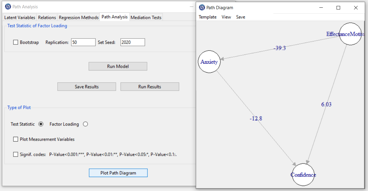
You can plot a path diagram by clicking this button. Before doing so, in the "Type of Plot" panel, you can specify the type and feature of the path diagram. In terms of path coefficient, there are two types of path diagrams:

Test Statistic: If this option is enabled, the coefficients in the path diagram will be the value of the statistic t or F (depending on the regression method). With these coefficients, you can decide whether the relationship between the variables is significant.

Factor Loading: If this option is enabled, loadings will appear in the outer model, and in the inner model, the coefficients of the regression model will appear.

*Plot Measurement Variables: If this option is disabled, only inner models will be the plot. But if this option is enabled, the outer model will be the plot. Note: If this option is enabled and we want to plot the path diagram based on the “Test Statistic”, the results must be executed (“RUN MODEL”) by activating the “Bootstrap” option.

*Signif. code: By activating this option, the path coefficients(Factor Loading or Test Statistic) will be displayed with a significant sign.

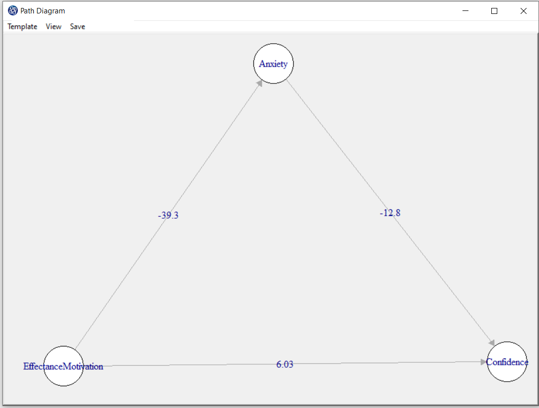
D8.5. Change Position in Path Diagram:

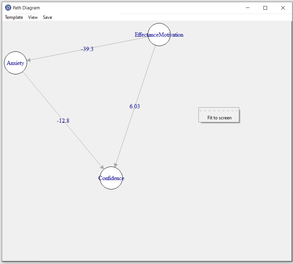
By opening the “Path Diagram” window, you can make the desired change on the path diagram. For example, you can change the size of this window and right-click and click on “Fit to Screen” to change the path diagram according to that size.
Also, you can change the position of each of the variables in the “Path Diagram” window.

D8.6. Path Diagram Size:

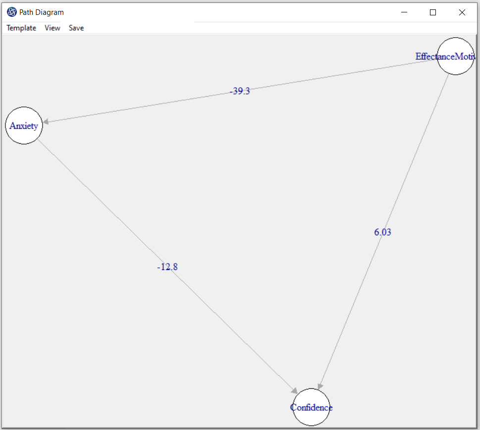
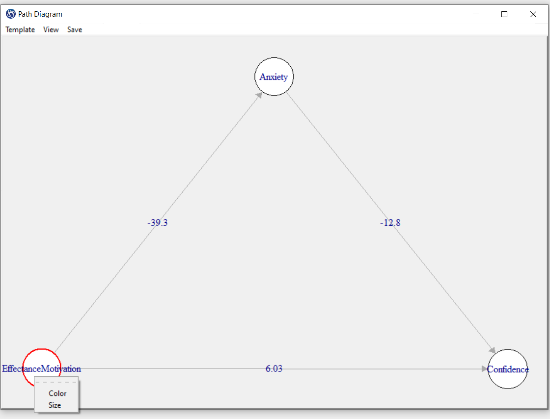
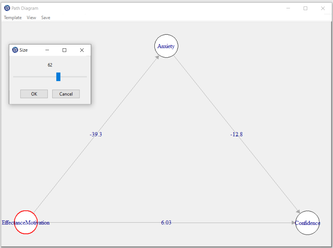
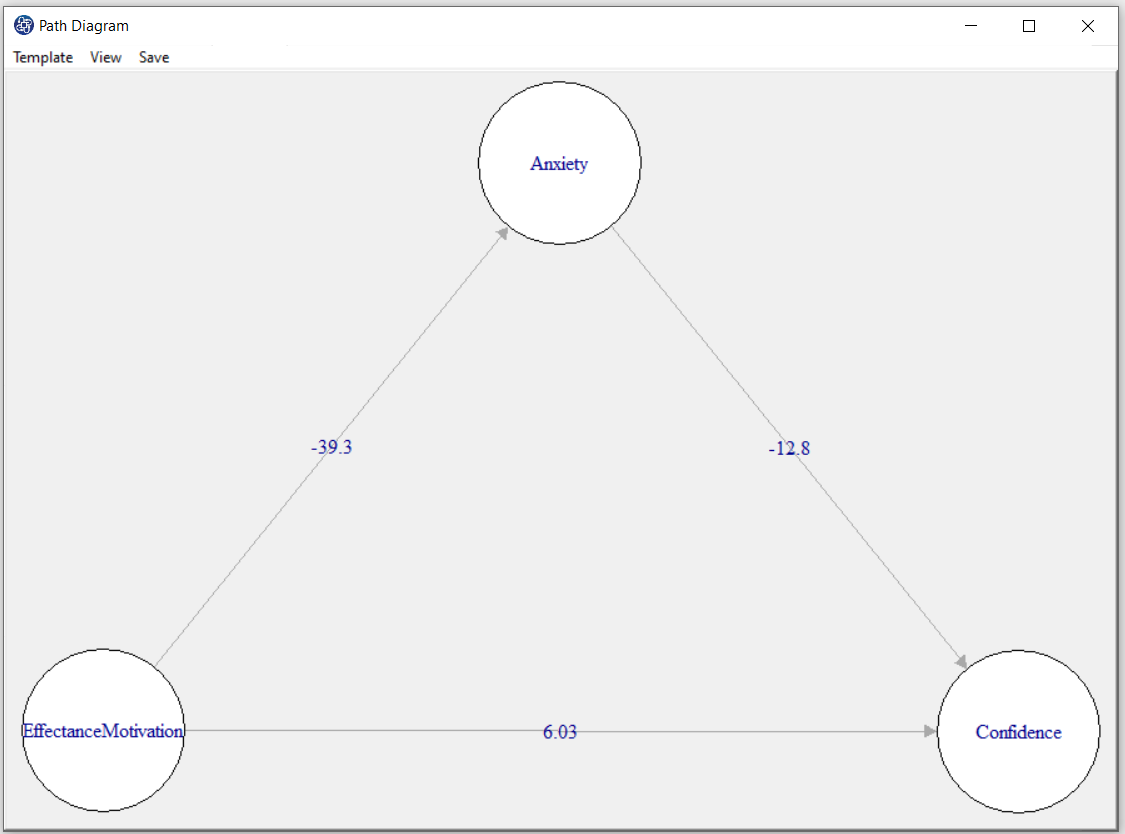
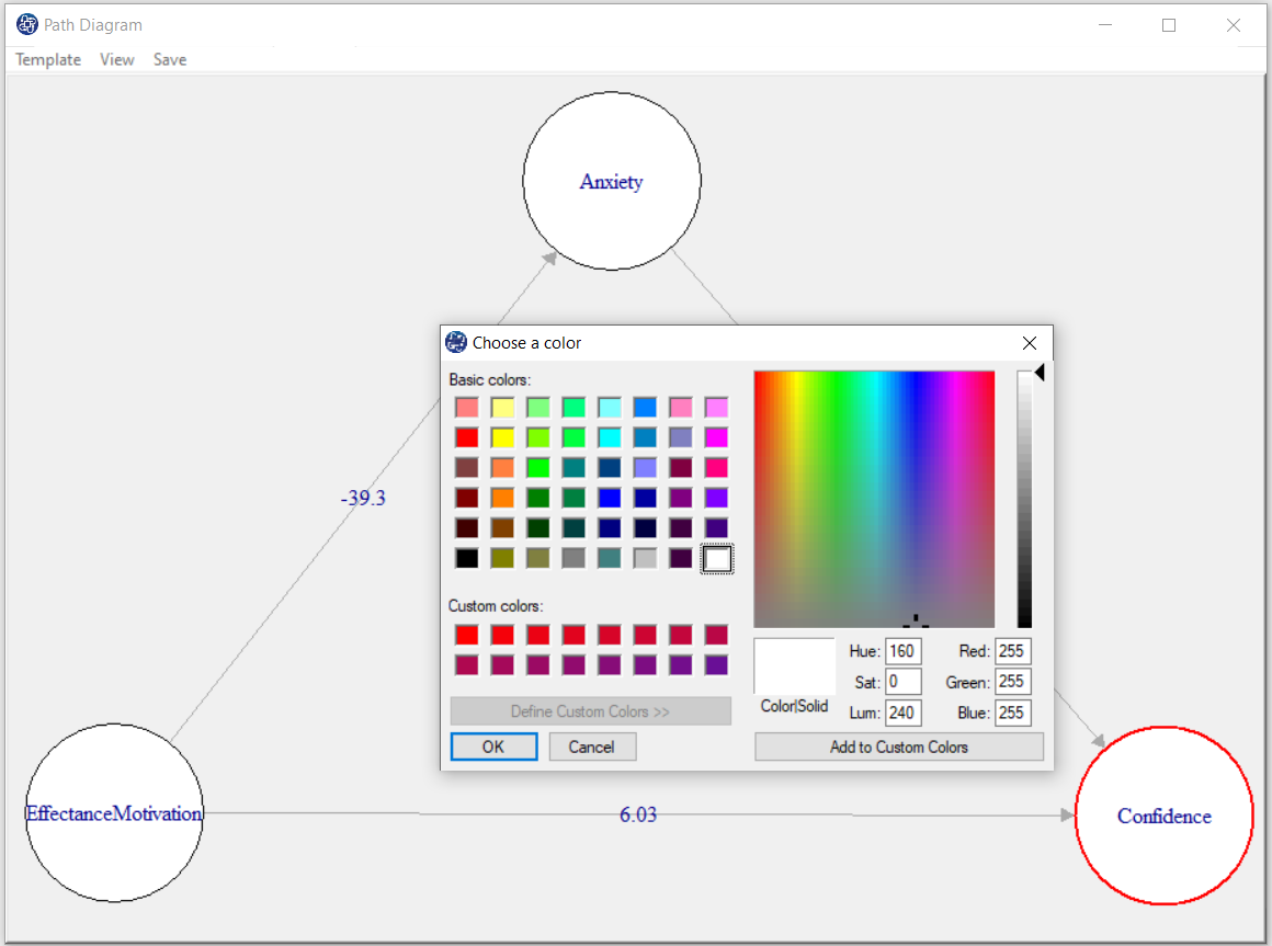
You can change the color and size in the path diagram. If you right-click on a circle or a line, you can change its size and color.
For example, we changed the size of the circle so that the titles of the variables fit inside the circle.

D8.7. Path Diagram Color:

Selecting the color after right-clicking on a circle or a line, the “Choose a color” will open. You can change the color by choosing the color you want.

D8.8. Template:

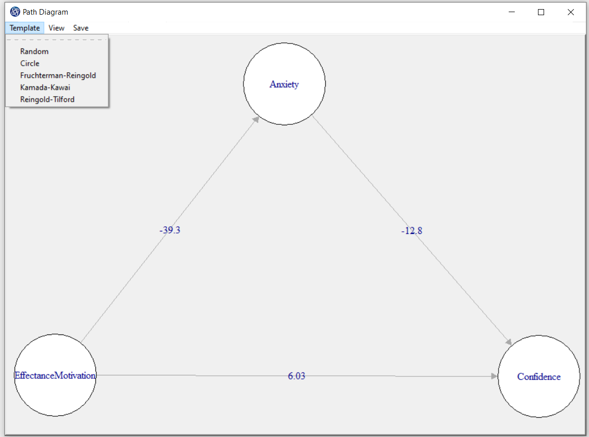
In Template, you can choose the layout of the path diagram using predefined patterns.

D8.9. View:

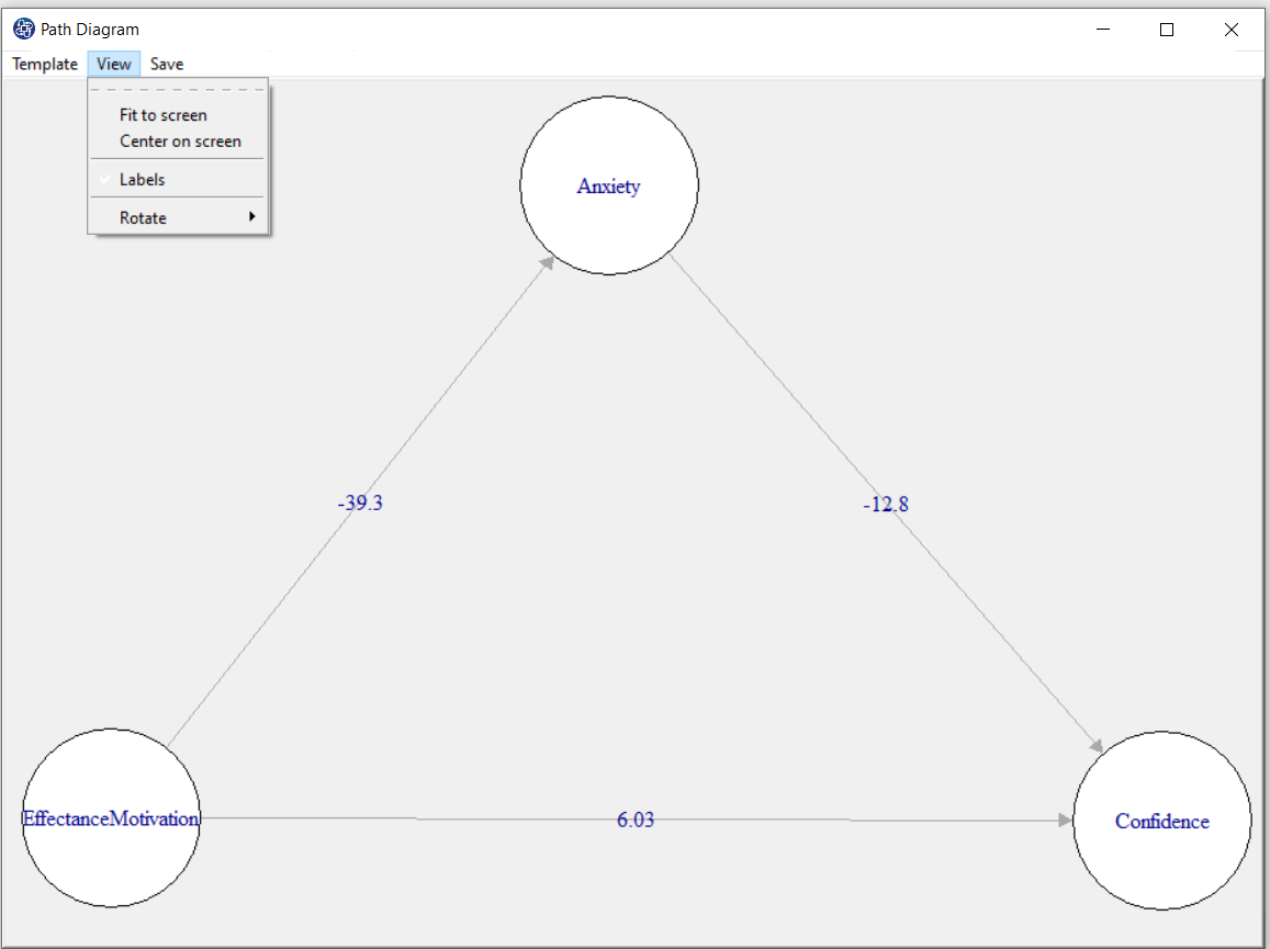
This option includes the following:

*Fit to Screen: Adjusts path diagram to the size of the "Path Diagram" window.

*Center on screen: The diagram puts the path in the center of the page.

*Labels: Show or hide labels in the path diagram.

*Rotate: Rotate the path diagram at the desired angle.

D8.10. Save:

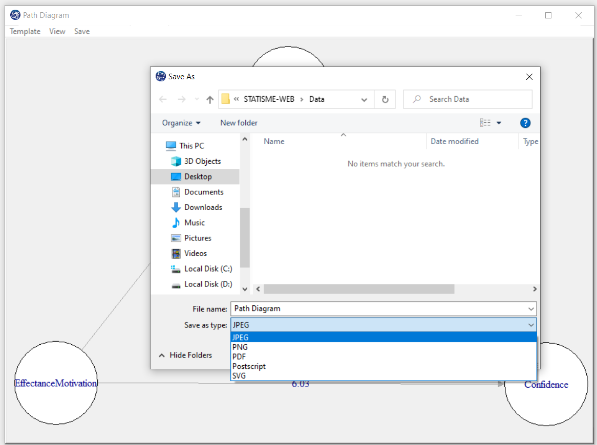
You can save the path diagram by clicking the Save in one of the following formats:
-JPEG
-PNG
-PDF
-Postscript
-BMP
-SVG

4.8.11. Type of plot(Plot Measurement Variables):

In the Type of Plot panel, you can specify the type and feature of the path diagram.
In terms of path coefficient, there are two types of path diagrams:

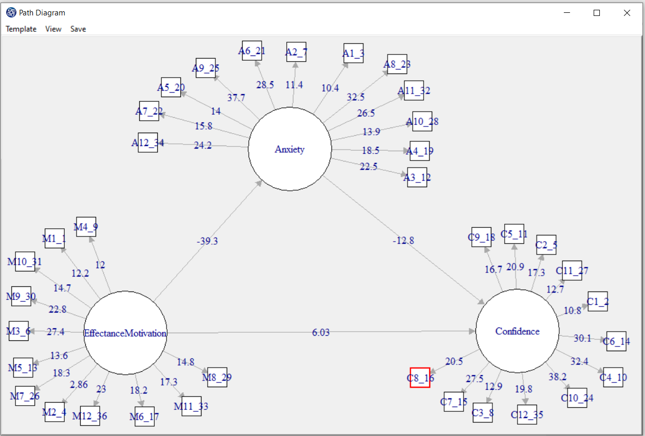
Test Statistic: If this option is enabled, the coefficients in the path diagram will be the value of the statistic t or F (depending on the regression method). With these coefficients, you can decide whether the relationship between the variables is significant.

Factor Loading: If this option is enabled, loadings in the outer model and the coefficients of the regression in the inner model will appear.

*Plot Measurement Variables: If this option is disabled, only inner models will be the plot. But if this option is enabled, the outer model will be the plot.
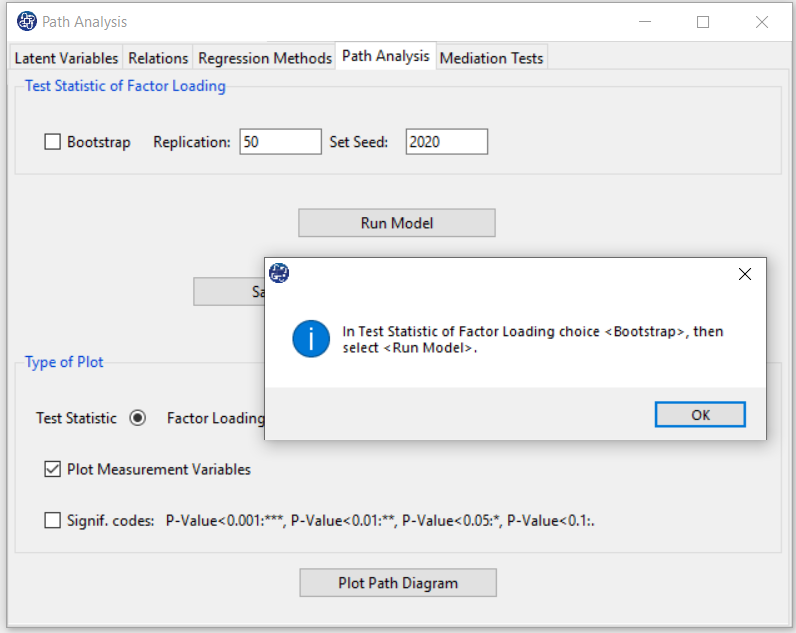
Note: If this option is enabled and we want to plot the path diagram based on the “Test Statistic”, the results must be executed (“RUN MODEL”) by activating the “Bootstrap” option.

4.8.12. Type of plot(Significant code):

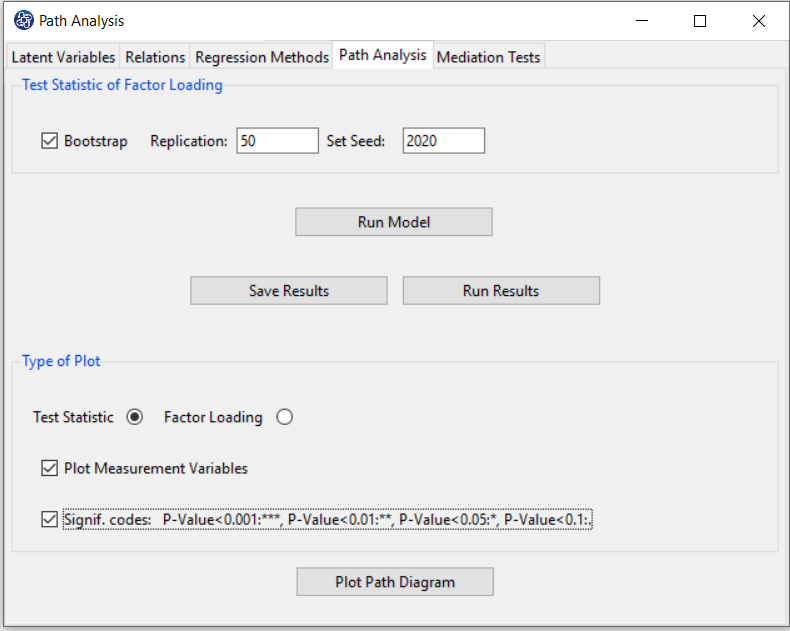
By activating “Signif. Code”, the path coefficients(Factor Loading or Test Statistic) will be displayed with a significant sign.

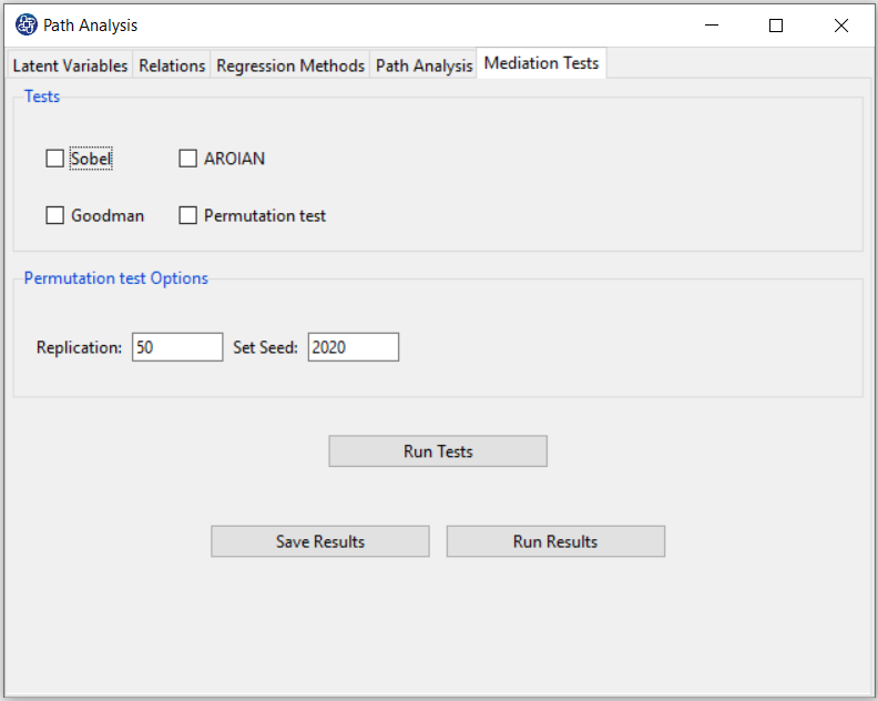
D9. Step 7.1. Mediation Tests:

If there is at least one indirect relationship in the model, you can use the tests in this tab to check the significance of the indirect relationship.
*Tests: In this panel, you can select the tests you want. You must choose at least one of “Sobel”, “AROIAN”, “Goodman” and “Permutation test” tests.

*Permutation test Options:
These options are used for the test via permutation, which includes the following:
*Replication: Number of Replication(B in equations).
*Set Seed: An arbitrary number will keep the Bootstrap results fixed by holding it fixed.
(See Introduction to SEM-PLS: E.4.1. Mediation Analysis)

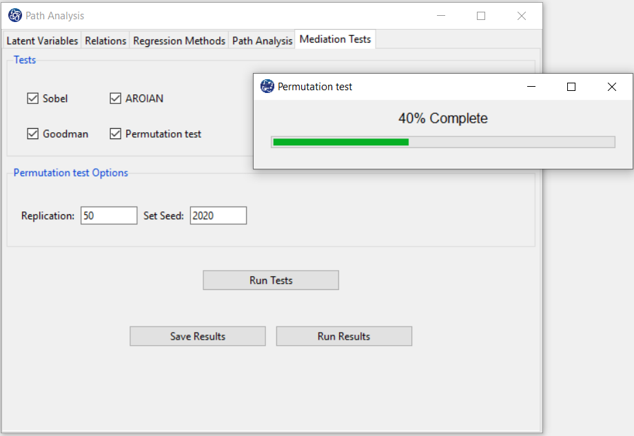
D9.1. Run Tests:

By clicking this button, you can test the mediation.
Note: Due to the “Permutation test” structure, this test requires more time than other tests. The percentage of progress of this test will be determined.

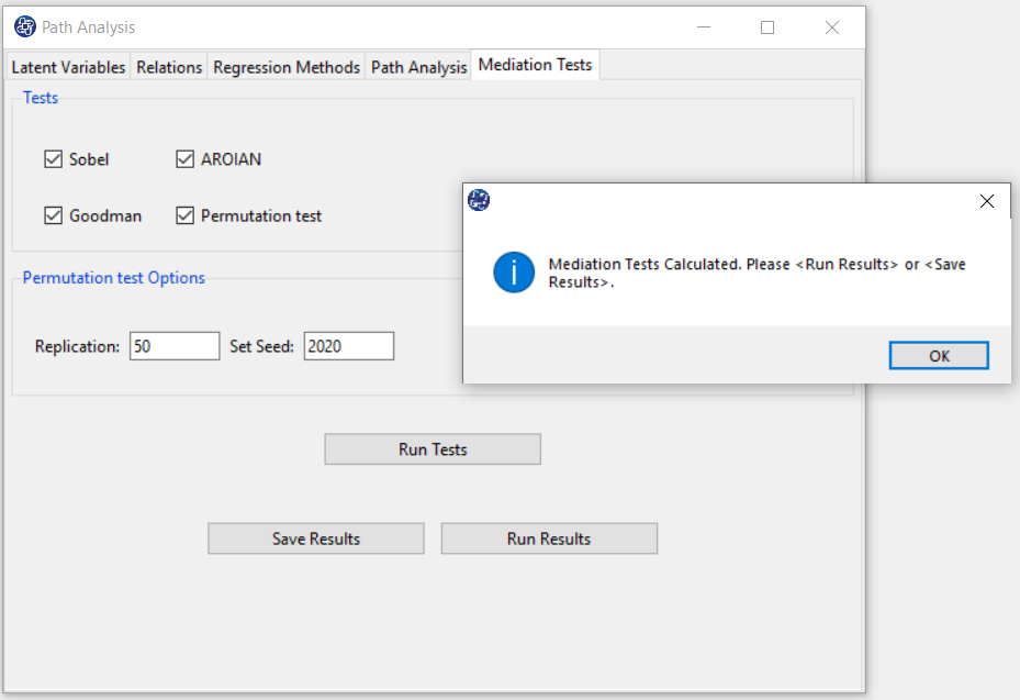
If the indirect relationships test is done without problems, this message appears:
“Mediation Tests Calculated. Please < Run Results> or < Save Results>.”

D9.2. Run Results:

After clicking on the “Run Results” button, for each indirect relationship, you can see the results of selected tests in the main software window.

D9.3. Save Results:

By clicking this button, you can save the mediation tests results. After opening the save results window, you can save the results in “text” or “Microsoft Word” format.

E. Model with Interaction Variable:

E.1: Add New Variable:

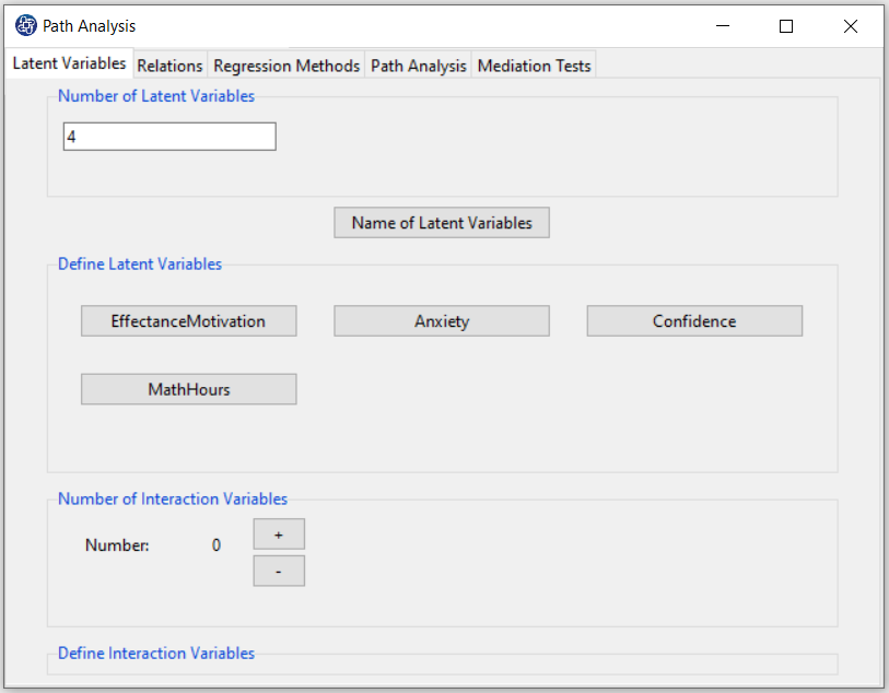
In the first step, you have to add one (or more) other variables like MathHours to the latent variables.
For this purpose, it increases the number of variables defined in Section D (for example, we change the number of variables from 3 to 4).
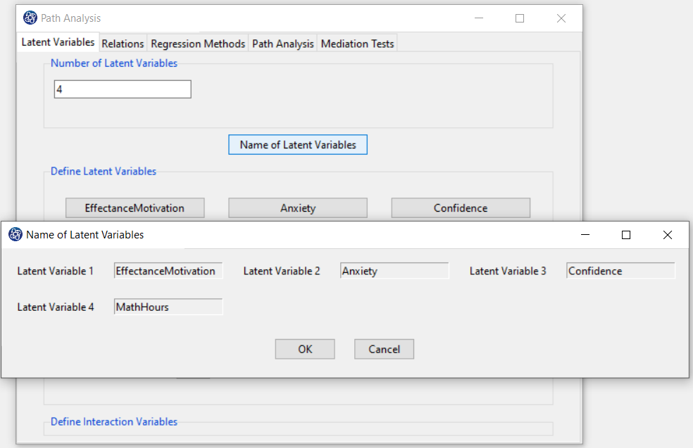
By clicking the “Name of Latent Variable” button, you can add the name of the added variable (or variables) to the other latent variables.
You can define the measurement variables corresponding to the added variable(s) in Define Latent Variables,.

E2. Step3.1:

In step 3.1, you must define the interaction variable:
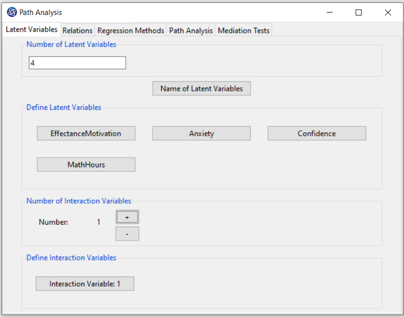
1-Number of Interaction Variables:
In this section you must specify the number of multiplicative variables.
You can increase or decrease the number of interaction variables with the + or - buttons, respectively.
With the increase (decrease) of variables, the number of buttons in the “Define Interaction Variables” panel will increase (decrease).
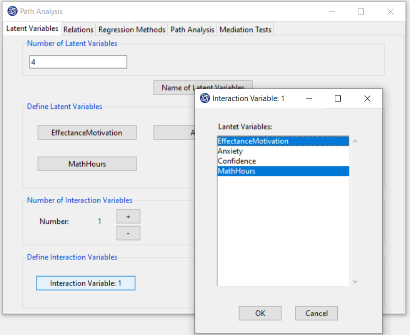
2-Define Interaction Variables:
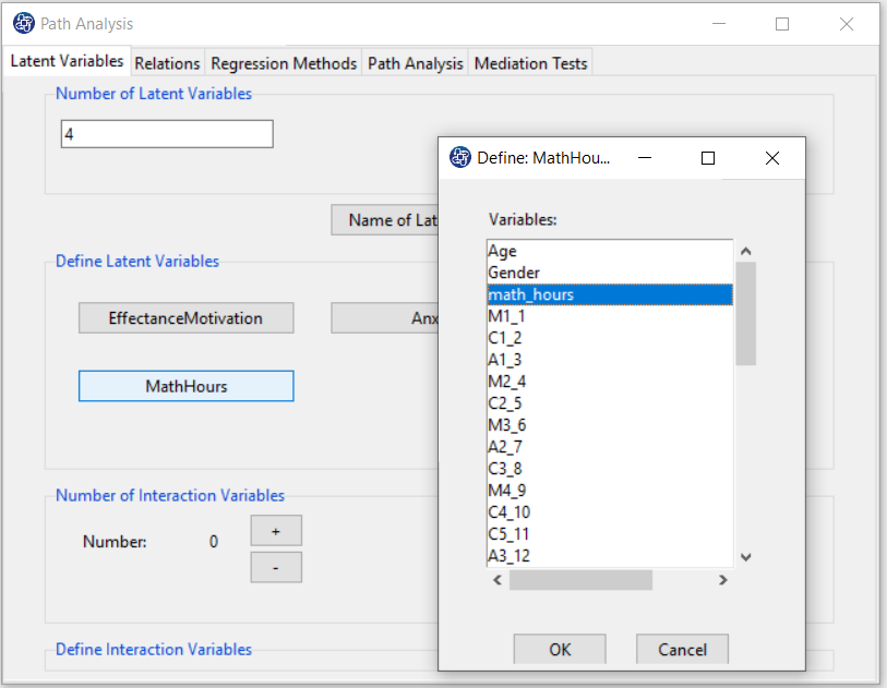
Click the “Interaction Variable:” button and select the multiplier variables from the defined latent variables.
For Example, you can define a new multiplicative variable with two variables, EffectanceMotivation and MathHours.

E2. Interaction Relation:

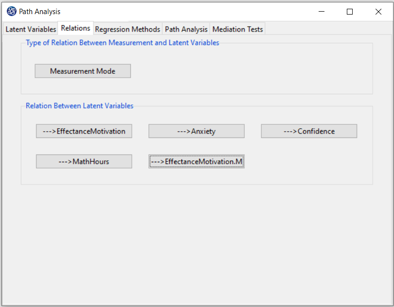
After defining the interaction variable(s) (multiplicative variable defined in the “Define Interaction Variables” panel), this variable(s) will appear in the “Relation Between Latent Variables” panel.
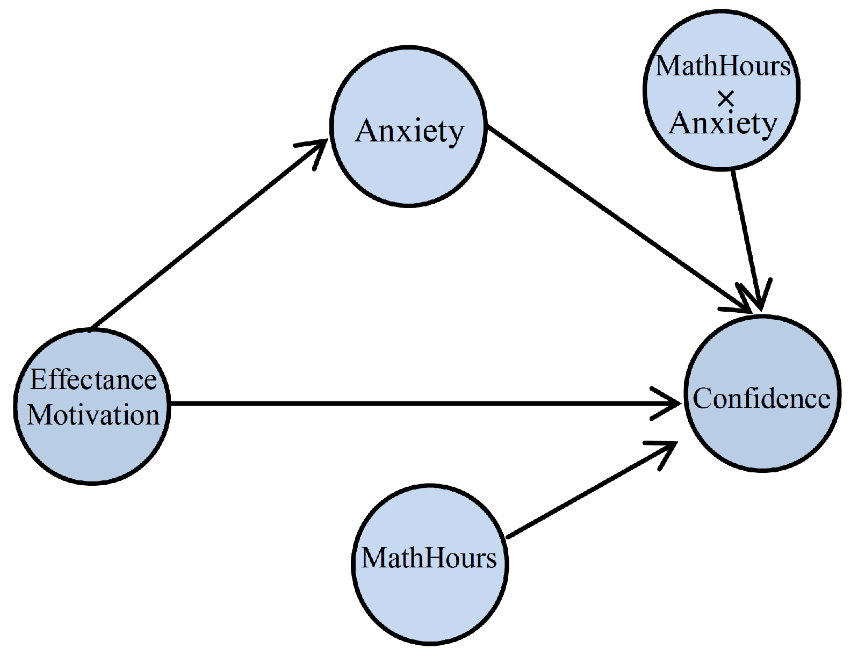
For example, after defining the “MathHours” variable and the “MathHours× EffectanceMotivation” multiplicative variable, these two variables have been added to the “Relation Between Latent Variables” panel.
You can define these variables in the model. For example, you can change the conceptual model as follows:


Thus, you will have the following two regression models to fit this conceptual model to the data:

E3. Results:

You can do steps 4 to 7.1, similar to section D.
In software results, the name of the interaction variable consists of the names of two variables with a dot placed between the two names. For example: