Multinomial Regression

Example Variables(Open Data):

The Fennema-Sherman Mathematics Attitude Scales (FSMAS) are among the most popular instruments used in studies of attitudes toward mathematics. FSMAS contains 36 items. Also, scales of FSMAS have Confidence, Effectance Motivation, and Anxiety. The sample includes 425 teachers who answered all 36 items. In addition, other characteristics of teachers, such as their age, are included in the data.
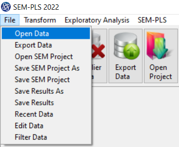
You can select your data as follows:
1-File
2-Open data
(See Open Data)

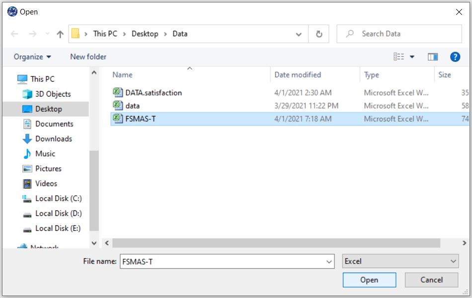
The data is stored under the name FSMAS-T(You can download this data from here ).
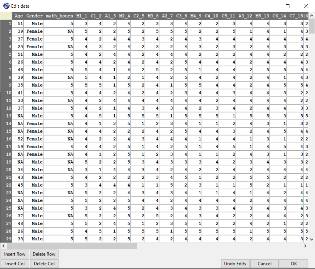
You can edit the imported data via the following path:
1-File
2-Edit Data
(See Edit Data)

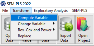
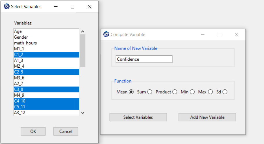
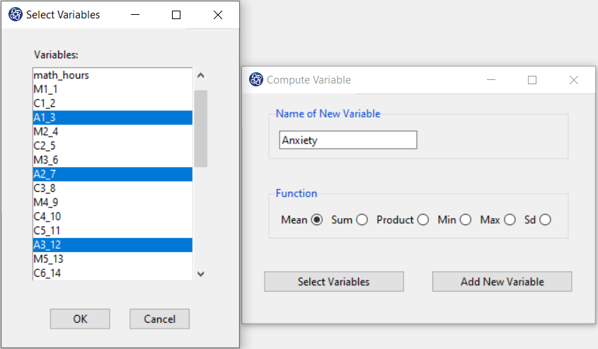
Example Variables(Compute Variable):

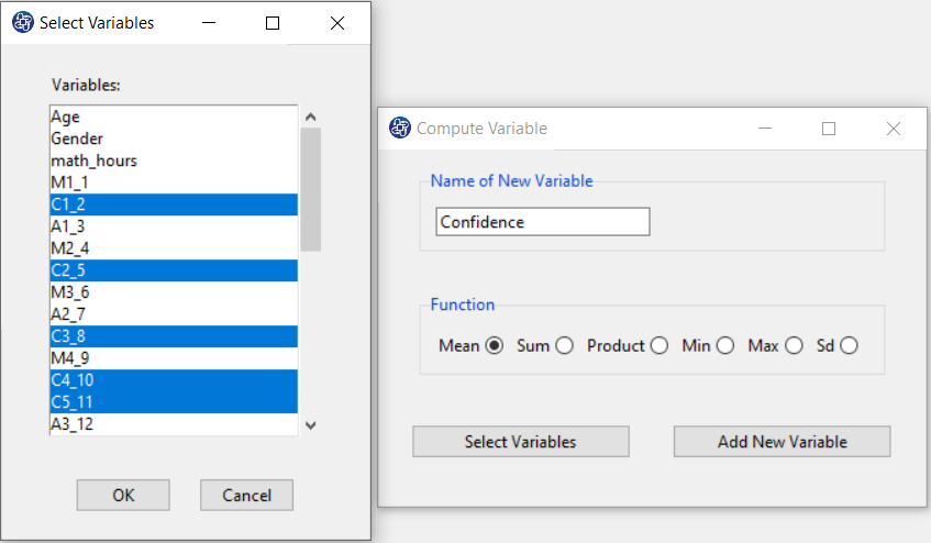
The three variables of Confidence, Effectance Motivation, and Anxiety can be calculated through the following path:
1-Transform
2-Compute Variable
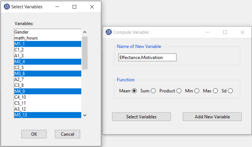
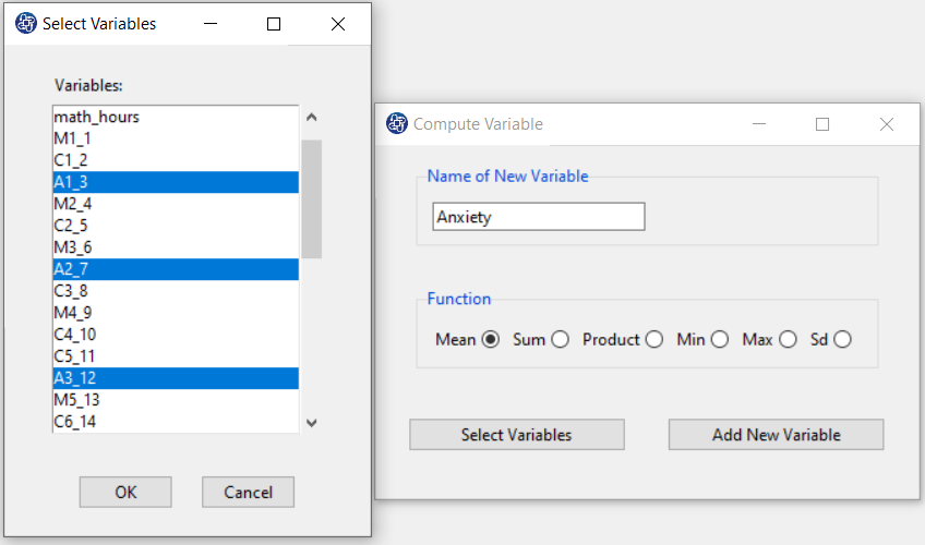
Items starting with the letters C, M, and A are related to the variables Confidence, Effectance Motivation, and Anxiety, respectively.
(See Compute Variable)

Example Variables(Compute Variable):

Introduction to Multinomial Regression

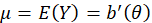
In many regression problems, the dependent variable is restricted to a fixed set of possible values. The multinomial logit model is the most widely used regression model that links a categorical dependent variable with unordered categories to independent variables. Let denote the dependent variable in categories , the multinomial logit model uses the same linear form of logits. But instead of only one logit, one has to consider logits. One may specify
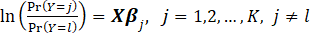
Where is called Reference Level or Reference category.

Therefore, the parameters can also be estimated by fitting a binary logit model using only observations in categories and . In fact, we have with GLM Regression that link function and distribution are Logit and binomial, respectively.

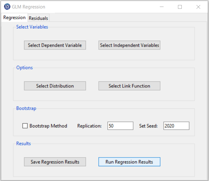
*A brief description of GLM Regression:

Most of the commonly used statistical distributions are members of the exponential family of distributions whose densities can be written in the form 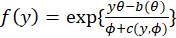Where is the dispersion parameter and is the canonical parameter. It can be shown that

A single algorithm can be used to estimate the parameters of an exponential family glm using maximum likelihood.
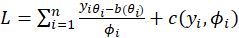
The log-likelihood for the sample is
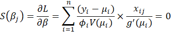
For ,the maximum likelihood estimates are obtained by solving the score equations
We assume that , Where are known prior weights.
A general method of solving score equations is the iterative algorithm Fisher’s Method of Scoring. In the r-th iteration, the new estimate is obtained from the previous estimate . After calculations, is obtained from the following relation:

i.e. the score equations for a weighted least squares regression of on withs , Where

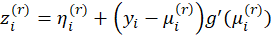
Hence the estimates can be found using an Iteratively Weighted Least Squares algorithm:
1-Start with initial estimates
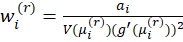
2-Calculate working responses and working weights
3-Calculate by weighted least squares
4-Repeat 2 and 3 till convergence
or models with the canonical link, this is simply the Newton-Raphson method.
The estimates have the usual properties of maximum likelihood estimators. In particular, is asymptotically .

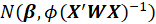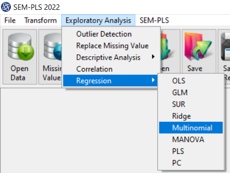
Path of Multinomial Regression:

You can perform Multinomial regression by the following path:
1-Exploratory Analysis
2- Regression
3-Multinomial

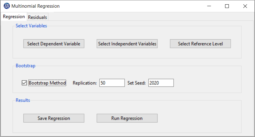
A. Multinomial Regression window:

Multinomial Regression window includes two tabs, Regression and Residuals.

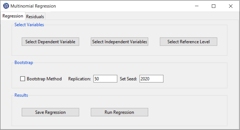
B. Regression

B1. Select Dependent Variable:

You can select the dependent variable through this button. After opening the window, you can select it by selecting the desired variable.
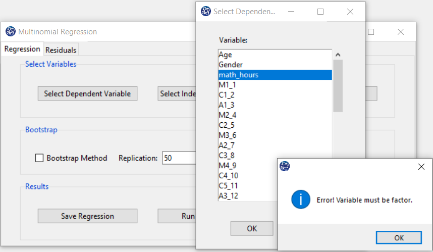
For example, the variable math_hour is selected in this data.
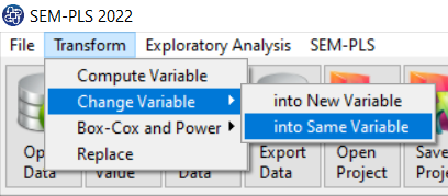
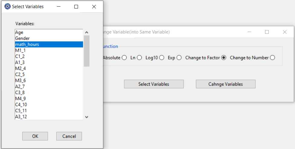
When selecting a dependent variable, you may encounter the problem that the selected variable is not factor. You can convert the dependent variable to factor through Change Variable> into Same Variable menu and by selecting Change to Factor function.

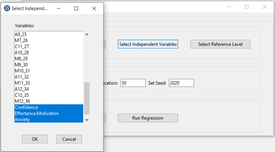
B2. Select Independent Variable:

You can select the independent variable through this button. After the window opens, you can choose them by selecting the desired variables. For example, the variables Confidence, Effectance Motivation and Anxiety are selected in this data.

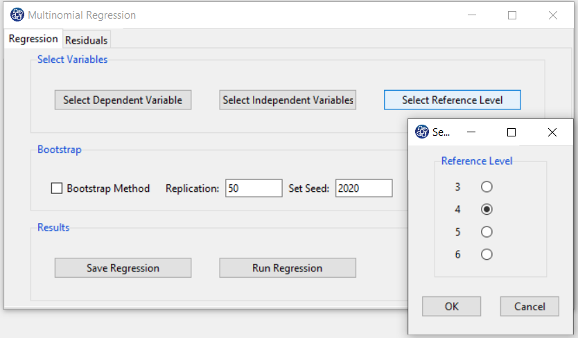
B3. Select Reference Level:

You can select one of the dependent variable levels as a Reference. For example, level 4 of the math_hour variable is selected as a Reference.

B3. Run Regression:

You can see the results of the Multinomial regression in the results panel by clicking this button.
Results include the following:
-Coefficients
-Model Summary

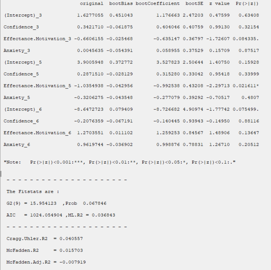
B3.1. Results:

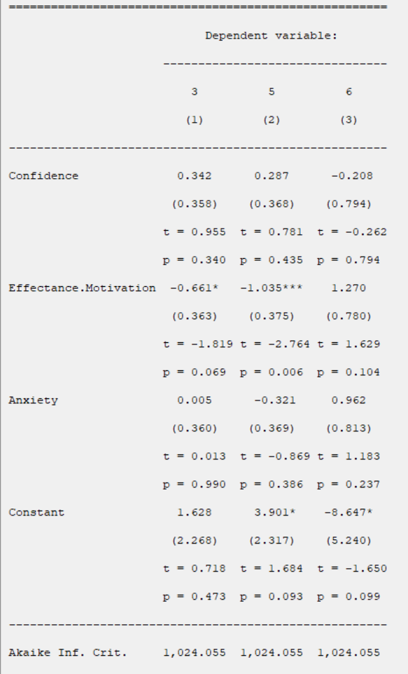
Coefficients:
For each models, the coefficients presented in this table are obtained from the following relationships, respectively:

*Beta:
For example, coefficients of the Confidence variable for levels 3, 5, and 6 are 0.342, 0.287, and -0.208 respectively.

*Std. Error:

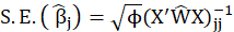
For example, the standard error of the Confidence variable for levels 3, 5, and 6 are 0.342, 0.287, and -0.208 respectively.

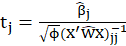
*t:
For non-Normal data, we can use the fact that asymptotically.

*p:
P-Value=Pr(| |>z)
Note: Constant represents the constant coefficient of the model.

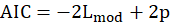
*AIC:
The deviance of a model is defined as 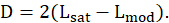. Where is the log-likelihood of the fitted model and is the log-likelihood of the saturated model.
The Saturated Model is a model that assumes each data point has its own parameters (which means you have n parameters to estimate.)
The AIC is a measure of fit that penalizes for the number of parameters p

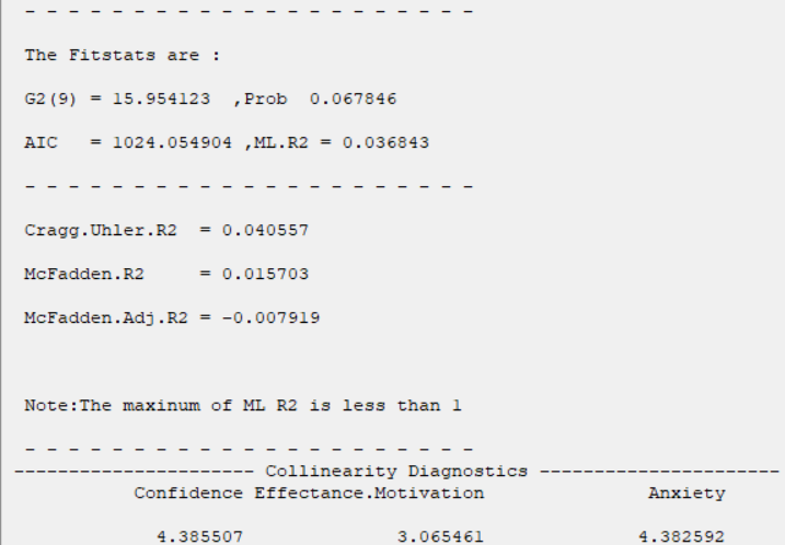
*G2 and Prob:
The likelihood-ratio statistic is 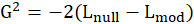Where is the log-likelihood of the fitted model and is the log-likelihood of the constant model( ).
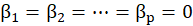and .

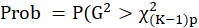
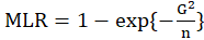
*ML.R2:
Maximum likelihood equals to Where is likelihood-ratio statistic.

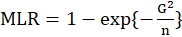
*Cragg.Uhler.R2:
Cragg&Uhler equals to Where is sample size, is the log-likelihood of the fitted model, is the log-likelihood of the constant model( .), and

*McFadden.R2:

McFadden equals to

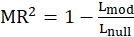
Where is the log-likelihood of the fitted model and is the log-likelihood of the constant model( .).

*McFadden.Adj.R2
Adjusted McFadden equals to 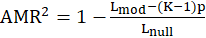Where is the log-likelihood of the fitted model, is the log-likelihood of the constant model( .), is the number of independent variables, and K is the number of categories of dependent variables.

*Collinearity Diagnostics:
In the Collinearity Diagnostics table, the results of multicollinearity in a set of multiple regression variables are given.
For each independent variable, the VIF index is calculated in two steps:
STEP1:
First, we run an ordinary least square regression that has x_i as a function of all the other explanatory variables in the first equation.
STEP2:
Then, calculate the VIF factor with the following equation: Where is the coefficient of determination of the regression equation in step one. Also,
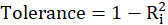
A rule of decision making is that if then multicollinearity is high (a cutoff of 5 is also commonly used)

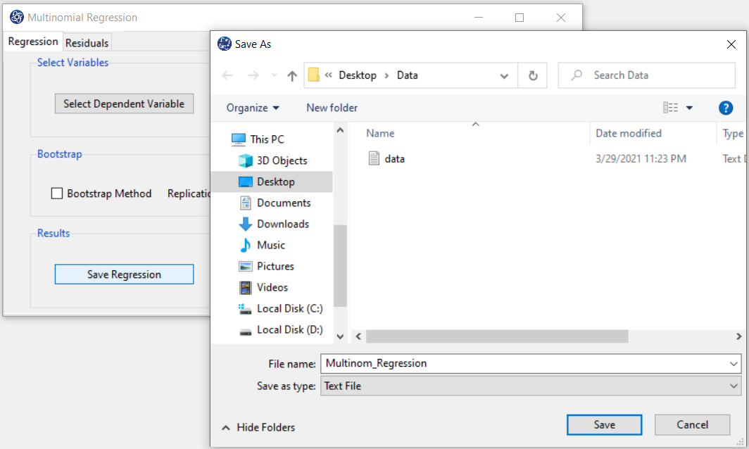
B4. Save Regression:

By clicking this button, you can save the regression results. After opening the save results window, you can save the results in “text” or “Microsoft Word” format.

B5. Bootstrap:

This option is located in the Regression tab. This option includes the following methods:
Assume we want to fit a regression model with dependent variable y and predictors x₁, x₂,..., x_p. We have a sample of n observations z_i = (y_i, x_i1, x_i2,...,x_ip) where i= 1,...,n. In random x resampling, we simply select B(Replication) bootstrap samples of the z_i, fitting the model and saving the and and from each bootstrap sample. The statistic t is normally distributed (which is often approximately the case for statistics in sufficiently large Replication ). If is the corresponding estimate for the ith bootstrap replication and is the mean of the s ,then the bootstrap estimation and the bootstrap standard error are

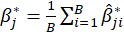
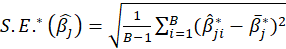
Thus

*Bootstrap Method:
Enabling this option means performing regression using the bootstrap method with the following parameters:

*Replication: Number of Replication(B in equations)

*Set Seed: It is an arbitrary number that will keep the Bootstrap results fixed by holding it fixed.

B5.1. Result(Bootstrap):

Running regression with the Bootstrap option enabled provides the following results:
Original:
bootCoefficient:
bootBias:
bootSE:
z value: z value

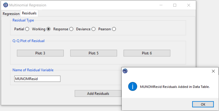
C. Residuals

C1. Residual Type:

In the Residual tab, the Residual Type option includes a variety of residues. Several kinds of residuals can be defined for GLMs:
*Partial: Partial residuals plots are similar to plotting residuals against , but with the linear trend with respect to added back into the plot.

*working: from the working response in the IWLS algorithm.

*response:

*Deviance:

*Pearson:

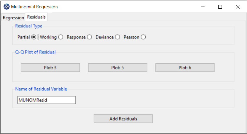
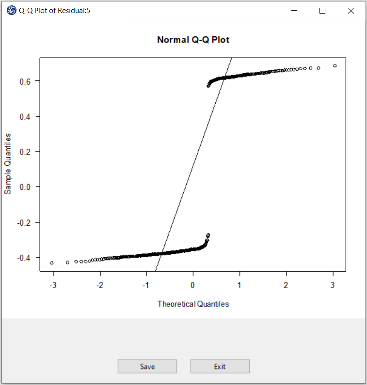
C2. QQ Plot of Residuals:

For each Model, after selecting the Residual Type, by clicking on the QQ Plot of Residuals button, You can assess the normality of the residues.
If the residuals follow a normal distribution with mean and variance ,then a plot of the theoretical percentiles of the normal distribution(Theoretical Quantiles) versus the observed sample percentiles of the residuals(Sample Quantiles) should be approximately linear. If a Normal QQ Plot is approximately linear, we proceed assuming that the error terms are normally distributed.

C3. Add Residuals & Name of Residual Variable:

By clicking on this button, you can save the Residuals of the regression model with the desired name(Name of Residual Variable). The default software for the residual names is “MUNOMResid”.
This message will appear if the Residuals are saved successfully:
“ Name of Residual Variable Residuals added in Data Table.”
For example,“MUNOMResid Residuals added in Data Table.”.