Introduction

Structural Equation Model based on Partial Least Squares (SEM-PLS) has been proposed different from the classic covariance-based LISREL approach.
SEM-PLS is considered a soft modeling approach where no strong assumptions, with respect to the distributions, the sample size, and the measurement scale are required. SEM-PLS follows the SEM notations and symbols, including the use of a path diagram to picture the relationships among the LVs(Latent Variables) and between each MV(Measurement Variable) and the corresponding LV.
An SEM-PLS model is made up of two elements, the outer model (also called the measurement model), which describes the relationships between the MVs and their respective LVs, and the inner model (also called the structural model), which describes the relationships between the LVs.
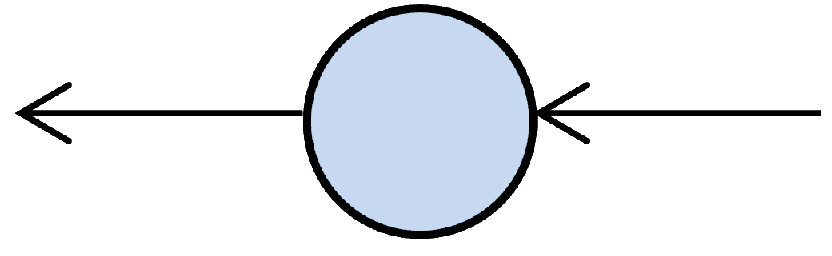
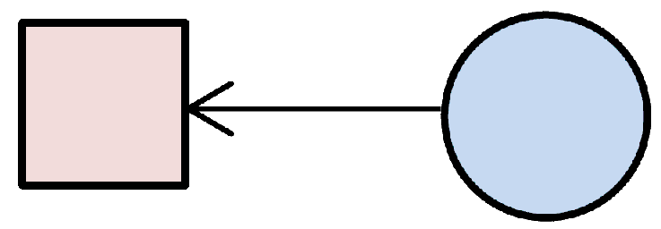
Structural equation models are schematically portrayed using particular configurations of three geometric symbols circle, square, and single-headed arrow. By convention, circles represent LVs, squares represent MVs, and single-headed arrows represent the impact of one variable on another. In building a model of a particular structure under study, researchers use these symbols within the framework of four basic configurations, each representing an essential component in the analytic process. These configurations, each accompanied by a brief description, are as Table1.

A. The Outer Model (The Measurement Model)

An LV is an unobservable variable (or construct) indirectly described by a block of observable variables called MVs. There are two ways to relate the MVs to their LVs:
1-The reflective (mode A)
2-The formative (mode B)

A.1. The reflective (mode A)

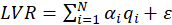
In the reflective way, each MV reflects the corresponding LV. A block is defined as reflective. This implies that the relationship between each MV and the corresponding LV is modeled as:



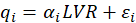
Where is the simple regression coefficient between the MV and the LV.
For example, a reflective way with four MVs can be considered in Figure 1.


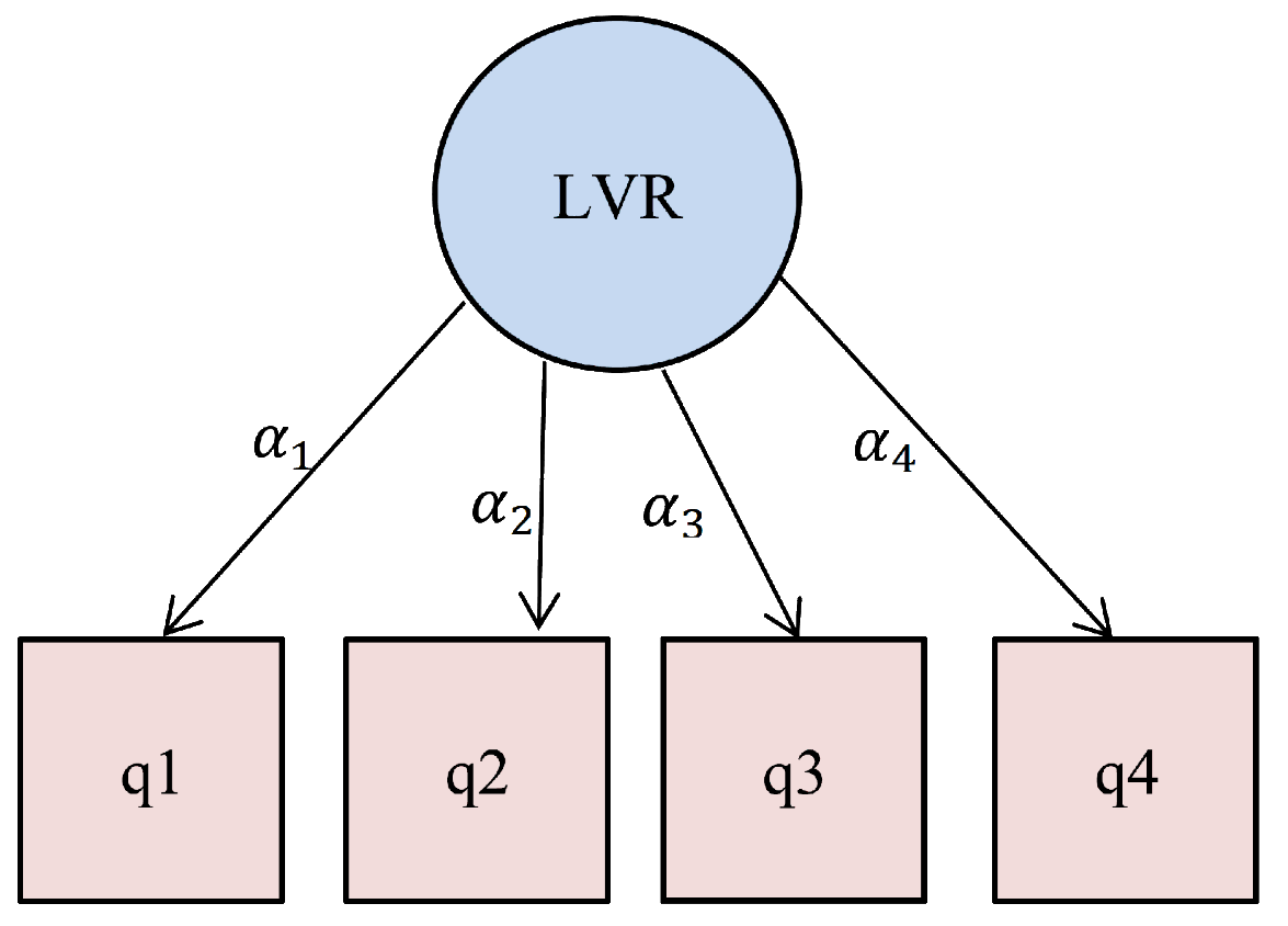
Figure 1: Reflective model with four MVs

A.2. The formative (mode B)

In the formative, the LV is supposed to be generated by its own MVs:



Where is the simple regression coefficient between the MV and the LV and is the number of MVs in the block of latent variables.
For example, a formative way with four MVs can be considered as Figure 2.


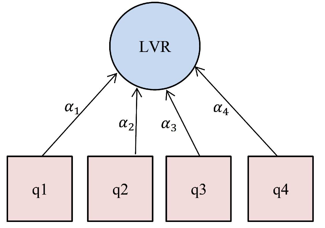
Figure 2: formative way with four MVs

B. The Inner Model (The Structural Model)

The structural model or Inner Model specifies the relationships between the LVs. If it is supposed to depend on other LVs, an LV is called dependent, and, otherwise, independent. In the structural model each independent LV is linked to the other LVs by the following multiple regression model. For Example, for , , , and , the path diagram is shown in Figure 3. For this model, the regression relations are:








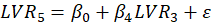
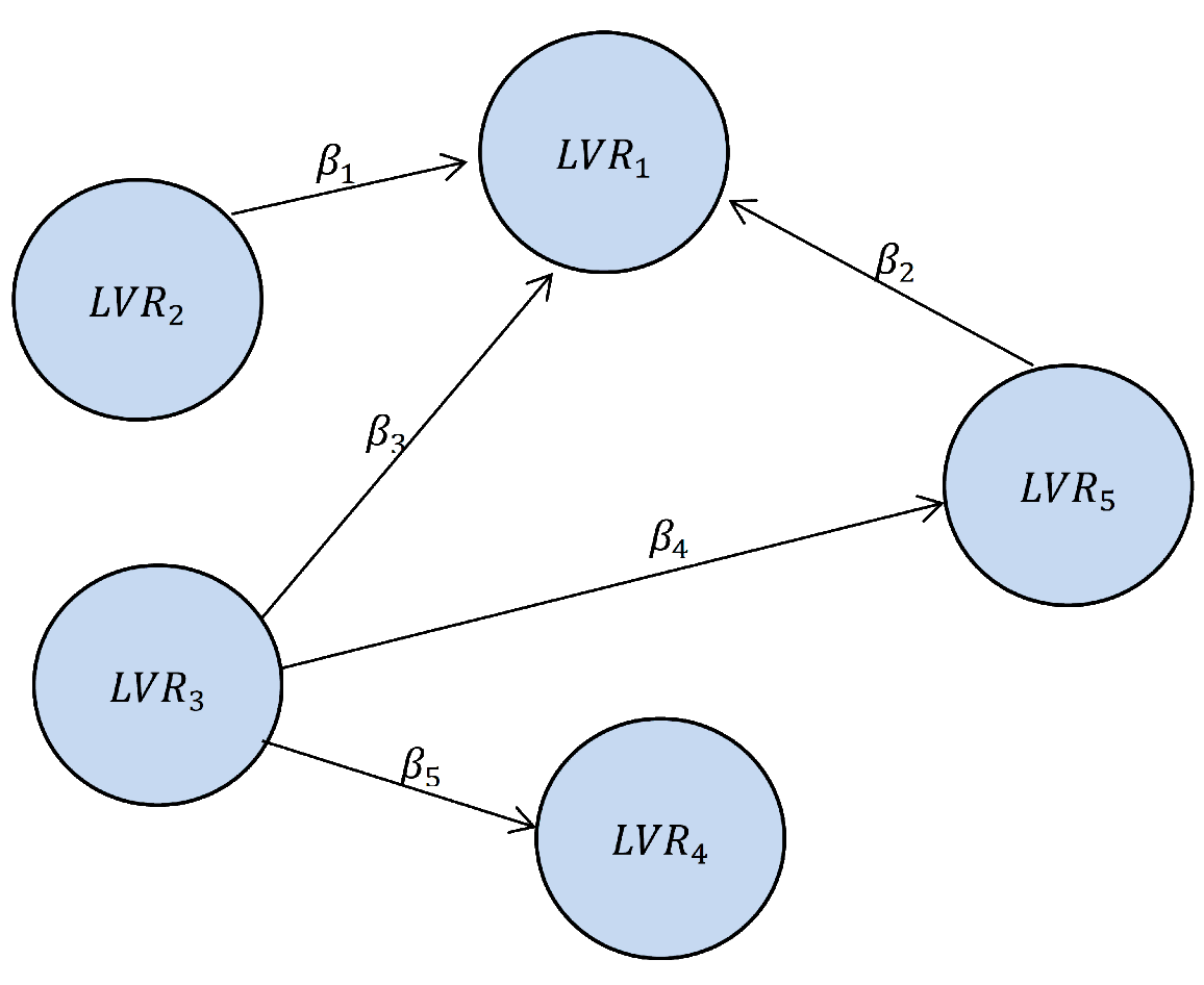
Figure 3: Example of path diagram of the inner model with five LVs.

C. SEM-PLS Algorithm

The SEM-PLS algorithm includes four stages:
1- Approximation of LVs
2- Estimation of the LVs scores
3- Loadings calculation
4- Estimation of the path coefficients

C.1. Approximation of LVs

The first stage of the algorithm consists of four steps
Step1: Initial arbitrary assignment of outer weights;
Step2: Computing the external approximation of the LVs and obtaining the inner weights;
Step3: Computing the internal approximation of the LVs;
Step4: Calculating the new outer weights;
Step5: Repeating step 2 to step 4 until convergence of the outer weights.

C.2. Estimation of the LVs scores

Once the final weights are obtained, the LVs scores are finally calculated as normalized weighted aggregates of the MVs.

C.3. Loadings calculation

The third stage of the algorithm consists of calculating the loadings. For convenience and simplicity reasons, loadings are preferably calculated as correlations between a latent variable and its MVs.
Also, Cross Loadings are the loadings of an MV with the rest of the latent variables.

C.4. Estimation of the path coefficients

In the last stage of the SEM-PLS algorithm, the path coefficients are estimated through one of the regression methods among the estimated LV scores, according to the path diagram structure.

D. Sample Size

One of the most fundamental issues in SEM-PLS is that of minimum sample size estimation. We can use one of three methods to determine the sample size:

D.1.The 10-Times Rule Method

The most widely used minimum sample size estimation method in SEM-PLS is the “10-times rule” method. Among the variations of this method, the one usually seen is based on the rule that the sample size should be greater than 10 times the maximum number of inner model links pointing at any latent variable in the model. For example, in the model used in Figure 3, the 10-times rule method leads to the minimum sample size estimation of 30, regardless of the strengths of the path coefficients.

D.2.The Minimum Method

This method relies on a table listing minimum required sample sizes based on three elements. The first element of the minimum method is the maximum number of arrows pointing at a latent variable. The second is the significance level used that we consider being equal to 0.05.
The third is the minimum in the model. The sample size required for this method is presented in Table 2.

Table 2: Determination of sample size using Minimum Method

Maximum Number of Arrows Pointing at A Construct	The Minimum
	(0,0.1]	(0.1,0.25]	(0.25,0.50]	(0.75,1]
2	110	52	33	26
3	124	59	38	30
4	137	65	42	33
5	147	70	45	36
6	157	75	48	39
7	166	80	51	41
8	174	84	54	44
9	181	88	57	46
More than 9	189	91	59	48

D.3.The Inverse Square Root Method

This method uses the inverse square root of a sample’s size for standard error estimation. In this method, the sample size is determined based on the minimum path coefficient as follows:



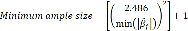
Where s are absolute of path coefficients and [x] gives as output the greatest integer less than x.

E. Validation of model

The evaluation of the inner and outer model results in SEM-PLS builds on a set of evaluation criteria.
Initially, the model assessment focuses on the outer models. When evaluating the outer models, we must distinguish between reflectively and formatively measured constructs. The criteria for reflective outer models cannot be universally applied to formative outer models. With formative measures, the first step is to ensure content validity before collecting the data and estimating the SEM-PLS. If the assessment of reflective and formative outer models provides evidence of the measures’ quality, the inner model estimates are evaluated. Hence, after the reliability and validity have been established, the primary evaluation criteria for the SEM-PLS results are the path coefficients, the coefficients of determination ( values), GOF, MSE, and …. The assessment of the SEM-PLS outcomes can be extended to more advanced analyses (e.g., multi-group testing, moderating effects and tests, REBUS, …). Therefore, there are three types of validation of models which must be done in order:
1- Validation of outer models
2- Validation of inner models
3- Extra Analysis

E.1.Validation of reflective outer models

The assessment of reflective outer models includes composite reliability to evaluate the internal consistency, individual indicator reliability, and Average Variance Extracted (AVE) to evaluate the convergent validity. In addition, the Fornell-Larcker criterion and cross loadings are used to assess the discriminant validity.

E.1.1. Reliability

In the reflective model, the MVs should be highly correlated, because they are correlated with the LV of which they are expressed. In other words, the block has to be homogeneous. There are several tools for checking the homogeneity of a reflective block:

Cronbach’s Alpha: A block is considered homogeneous if this index is larger than 0.7.



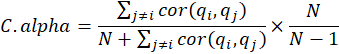
Where is the number of MVs in the block of latent variables. Cronbach’s Alpha is sensitive to the number of items in the scale and generally tends to underestimate the internal consistency and reliability.

Dillon- Goldstein’s Rho (Composite Reliability): This measures the composite reliability of the block. A block is considered homogeneous if its composite reliability is larger than 0.7.



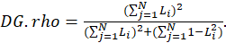
Where is the correlation between the MV and the LV (Loading) and is the number of MVs in the block of latent variables.

E.1.2. Convergent Validity

A common measure to establish convergent validity on the construct level is the AVE that expresses the degree of variance of the block explained by :



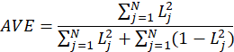
Where is the correlation between the MV and the LV (Loading) and is the number of MVs in the block of latent variables.
An AVE value of 0.5 or higher indicates that, on average, the construct explains more than half of the variance of its indicators. Therefore, the AVE is equivalent to the communality of a construct.
In a good outer model, each MV is well summarized by its own LV. So, for each block, a Communality Index is computed as:



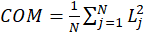
Where is the correlation between the MV and the LV(Loading) and is the number of MVs in the block of latent variables.

E.1.3. Discriminant validity

One method for assessing discriminant validity is by examining the cross loadings of the indicators. Specifically, an indicator’s outer loading on the associated construct should be greater than all of its loadings on other constructs.

The Fornell-Larcker criterion is another approach for assessing discriminant validity. It compares the square root of the AVE values with the LV correlations. Specifically, the square root of each construct’s AVE should be greater than its highest correlation with any other construct(see Table3).

Table3:FORNELL-LARCKER Matrix with four LVs Note: is of . is correlation of and .

E.2.Validation of formative outer models

We should focus on establishing content validity before empirically evaluating formatively measured constructs. This makes it necessary to ensure that the formative indicators capture all facets of the construct.

For evaluating formative outer models, we have to test whether the formatively measured construct is highly correlated with a reflective measure of the same construct. The strength of the path coefficient linking the two constructs is indicative of the validity of the designated set of formative indicators in tapping the construct of interest.

For example, Figure 4 shows the Convergent Validity for the two variables q1 and q2. If the analysis exhibits a lack of convergent validity ( is low) then the formative indicators of the construct do not contribute at a sufficient level to its intended content.

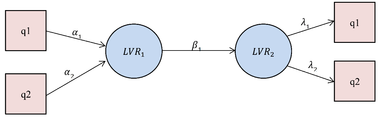
Figure 4: Convergent Validity Assessment(formative outer model)

This type of analysis is also known as redundancy analysis. Redundancy measures the percent of the variance of indicators in a dependent block that is predicted from the independent latent variables associated with the dependent LV. Another definition of redundancy is the amount of variance in a dependent construct explained by its independent latent variables. The redundancy index for the j-th MV in k-th dependent LV is:



Where is loading a reflective model, and is the coefficient of determination of LV. Also, redundancy of k-th dependent LV equals to



Where is the number of MVs in k-th dependent LV.

E.3. Validation of inner model:

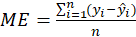
Once we have confirmed that the construct measures are reliable and valid, the next step addresses the assessment of the inner model results. This involves examining the model’s predictive capabilities and the relationships between the constructs. The key criteria for assessing the inner model in SEM-PLS are the significance of the path coefficients, the level of the , Cohen's , , ME, MSE, RMSE, MAE.

: This index is the coefficient of determination that how it is calculated depends on the Regression Method.

Cohen's : This index is obtained from the following equation:



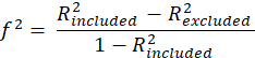
Where and are value of the dependent LV when a selected independent LV is included in or excluded from the model. Guidelines for assessing are proposed

Small impact:

Medium impact:

Large impact:

GOF: The GoF(Goodness Of Fit) can be proposed as the geometric mean of the average communality and the average of :



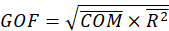
Where for dependent latent variables, and .
ME, MSE, RMSE and MAE: If and the value of dependent latent variable and the dependent variable predicted, respectively:

E.4. Extra Analysis

In mediation analysis, the relationship of the independent variable to the dependent variable is influenced by another LV called the Mediator Variable (See Figure 5). Therefore, in addition to the direct effect , we must also consider the indirect effects.

Mediator models can be divided into two types, Partial Mediation and Full Mediation.
In Partial Mediation, there is a direct relationship between two variables, while in Full Mediation, only the mediating variable determines the relationship between these two variables.

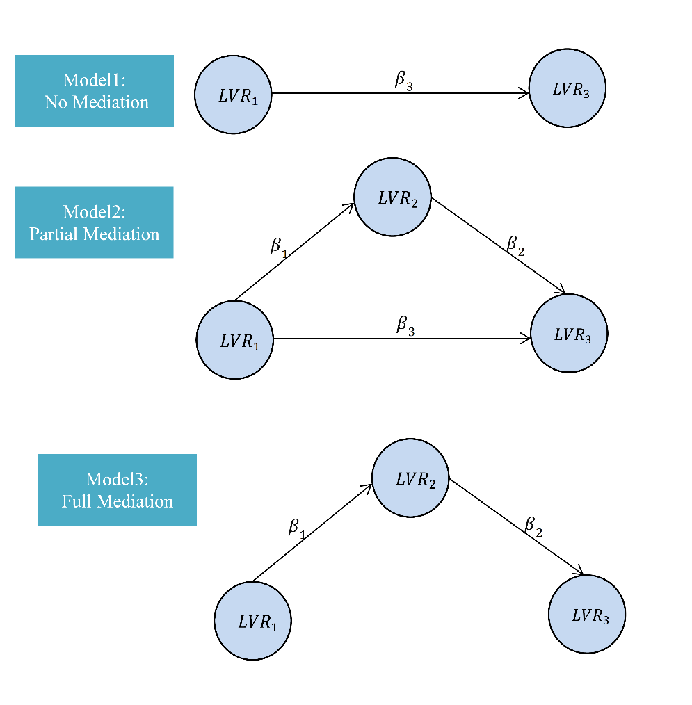
Figure 5: Mediator Models

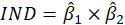
When including the mediator, the indirect effect must be significant. If the indirect effect is significant, the mediator absorbs some of the direct effect. The question is how much the mediator variable absorbs. To answer this question, the size of the indirect effect in relation equals to:
Consequently, tests must answer the following questions, is the indirect effect via the mediator variable significant after this variable has been included in the model?
To answer this question, the following mediation tests are provided:

E.4.1.1. Sobel Test, Aroian Test, and Goodman Test

Sobel Test, Aroin Test, and Goodman Test use the magnitude of the indirect effect compared to its estimated standard error of measurement to derive a statistic







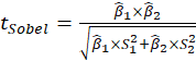
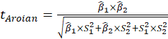
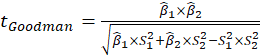
Where and are variance of and respectively. , and statistics can then be compared to the normal distribution to determine its significance.
However, these tests rely on distributional assumptions, which usually do not hold. Furthermore, these tests require unstandardized path coefficients as the input for the test statistics and lack statistical power, especially when applied to small sample sizes. The permutation test can be suggested to solve this problem.

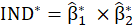
E.4.1.2. Permutation test

For B replication, the permutation test uses the following algorithm:

1- Model runs to obtain and an estimate for the real data and is calculated.

2- For each regression model, the dependent latent values are permuted randomly

3- Model runs to obtain and for the permuted data and is calculated.

4- Steps 2-3 are repeated number B of times.

5- Suppose


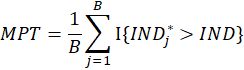
Where value of in j^th replication and function means if this function is equal to 1 and otherwise 0. The P-value of the permutation test is obtained from the following relation:

E.4.2. Moderator Analysis

Moderating effects are evoked by variables whose variation influences the strength or the direction of a relationship between independent and dependent variables (See Figure 6)

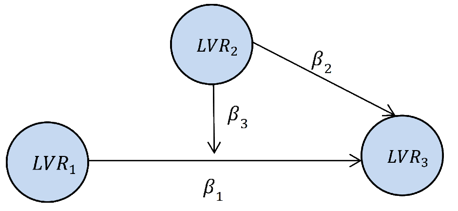
Figure 6: Model with a moderating effect

Basically, there are two main methods to study moderating effects depending on the nature of the moderator variable:

E.4.2.1. Moderator (Interaction) Constructs

This approach applies when the moderator variable is an LV; MVs of a latent moderator variable is observed and quantitative. Under this approach, moderator variables are considered in the inner model. In this method, the interaction variable

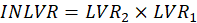
Basically, there are two main methods to study moderating effects depending on the nature of the moderator variable: is made by multiplying and i.e. . For example, if q1, q2 are MVs of , q3, q4 are MVs of , and q5, q6 are MVs of then the interactive model is shown in Figure 7. To calculate the interaction latent variable first MVs q1×q3, q1×q4, q2×q3, q2×q4 are calculated and then is created based on them.

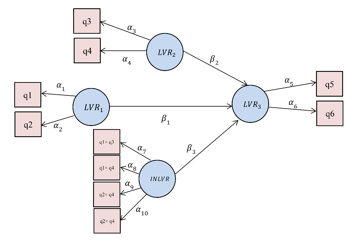
Figure 7: Model with a interaction variable

E.4.2.2. Group Analysis

This approach applies when the moderator is an observed MV, and it is a qualitative variable or can be categorized. In this case, the sample is split into two or more groups relating to the codes of the qualitative variable, and the path coefficient of the moderated relationship is estimated for each of the sub-samples. For Group Comparisons, Two types of tests are suggested:

E.4.2.2.1. t test

Suppose we have two groups and with path coefficients and , sample sizes of and , and Standard Errors of and , respectively. The formula that we use for the t-test statistic is:



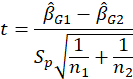
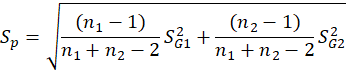
Where is the estimator of the pooled standard deviation and is obtained as follows:



Therefore, the P-value of this test is obtained from the following equation:



Where is the cumulative function of standard normal distribution.

However, these tests rely on distributional assumptions, which usually do not hold. In addition, this test can not test the difference between groups in , GOF, Cohen's , ME, MSE, RMSE and MAE indices. To solve this problem, the permutation test can be suggested.

E.4.2.2.2. Permutation test

Suppose is one of the (path coefficient), (loading), , GOF, Cohen's , ME, MSE, RMSE and MAE indices. we have two groups and with sample sizes of and , and Standard Errors of and and index of and . For B replication, the permutation test uses the following algorithm:

1- Model runs to obtain and for the real data and is calculated.

2- For each regression model, the dependent latent values are permuted randomly.

3- Model runs to obtain and for the permuted data and is calculated.

4- Steps 2-3 are repeated number B of times.

5- Suppose

 Where 


value of in j^th replication and function means if this function is equal to 1 and otherwise 0. The P-value of the permutation test is obtained from the following relation:

E.4.3. REBUS (Response Based Unit Segmentation)

Many datasets are far from being a homogenous mass of data. More often than not, you will find subsets of observations with a particular behavior; perhaps there is a subset that shows different patterns in the distribution of the variables, or maybe there are observations that could be grouped together and analyzed separately. It might well be the case that one single model is not the best model for your entire dataset, and you might need to estimate different path models for different groups of observations.

One of the traditional examples is when we have demographic information like gender, and we apply a group analysis between females and males. But what about those situations when we don’t have categorical variables to play with for multi-group comparisons? In these circumstances we could still apply a SEM-PLS analysis but we probably will be wondering “What if there’s something else? What if there’s something hidden in the data?

In this situation, we can use the REBUS method. REBUS is a technique inspired by cluster analysis techniques, and it applies clustering principles to obtain the solution. But don’t get confused. REBUS is not equivalent to cluster analysis. Although you could apply your favorite type of cluster analysis method to detect classes in your data, this is not what we are talking about.

REBUS uses the following algorithm:
1- Estimation of the Path Model.
2- Computation of the residuals of the model.
3- Perform a hierarchical clustering on the residuals computed in step 2.
4- Choose the number of classes K according to the dendrogram obtained in step 3.
5- Assignment of the observations to each group according to the cluster analysis results.
6- Estimation of the K local models.
7- K Groups are compared with one of the methods of Group Analysis (t test or Permutation test).