Example Variables(Open Data):

The Fennema-Sherman Mathematics Attitude Scales (FSMAS) are among the most popular instruments used in studies of attitudes toward mathematics. FSMAS contains 36 items. Also, scales of FSMAS have Confidence, Effectance Motivation, and Anxiety. The sample includes 425 teachers who answered all 36 items. In addition, other characteristics of teachers, such as their age, are included in the data.
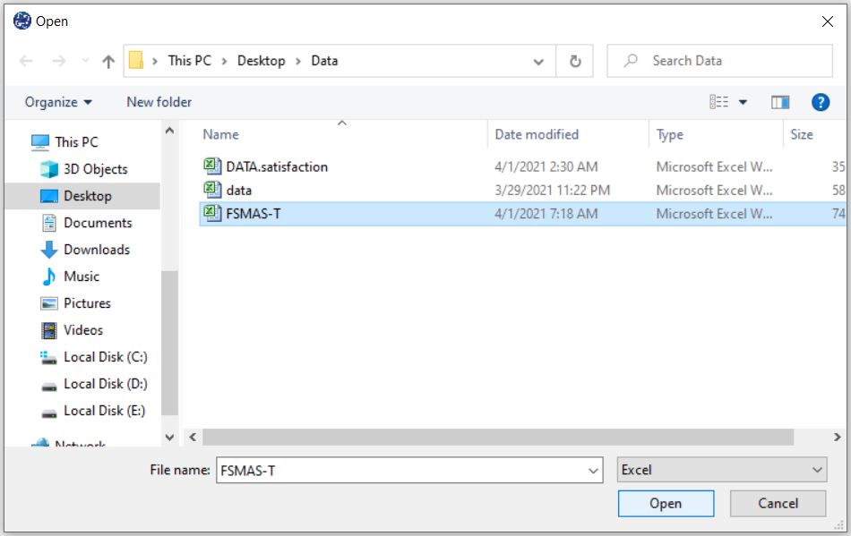
You can select your data as follows:
1-File
2-Open data
(See Open Data)

The data is stored under the name FSMAS-T(You can download this data from here ).
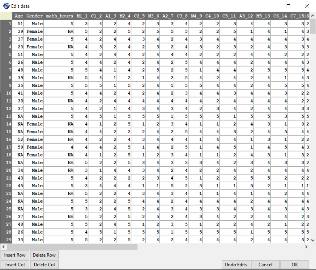
You can edit the imported data via the following path:
1-File
2-Edit Data
(See Edit Data)

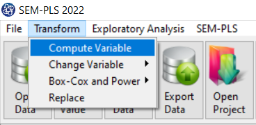
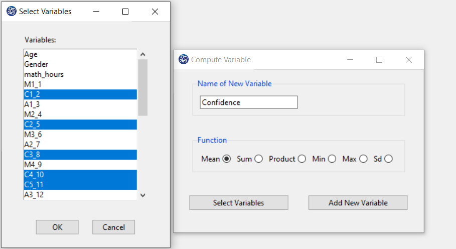
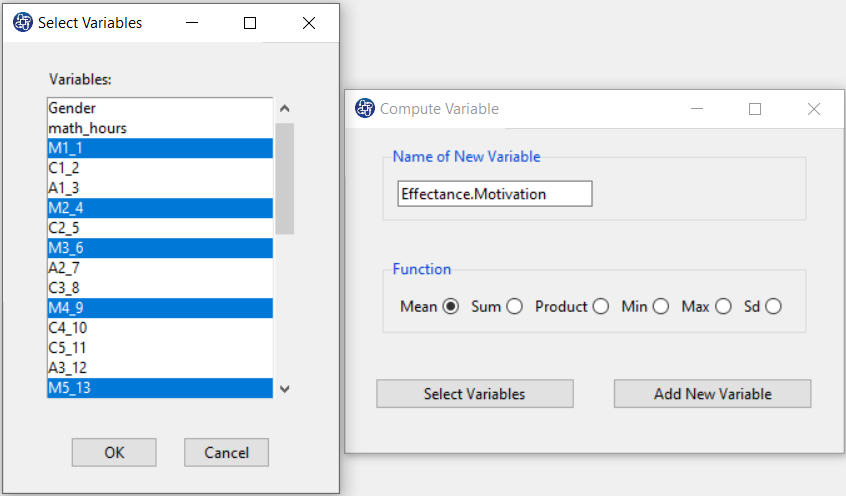
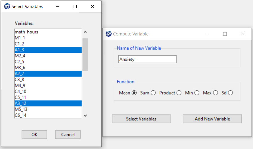
Example Variables(Compute Variable):

The three variables of Confidence, Effectance Motivation, and Anxiety can be calculated through the following path:
1-Transform
2-Compute Variable
Items starting with the letters C, M, and A are related to the variables Confidence, Effectance Motivation, and Anxiety, respectively.
(See Compute Variable)

Introduction to Ridge Regression

Suppose each observation i includes a scalar dependent variable y_i and column vector of values of p independent variables x_i1 , x_i2 , x_i3 ,…, x_ip .
A linear regression is a linear function of independent variables:

This model can also be written in matrix notation as

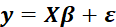
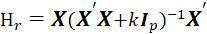
Where y and ε are n×1 vectors of the values of the response variable and the errors for the various observations, and X is a matrix. The ridge model coefficients are estimated as,

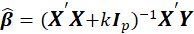
Where k is Ridge Biasing Parameter, at some values of k, the ridge coefficients get stabilized and the rate of change slow down gradually to almost zero. Therefore, a disciplined way of selecting the shrinkage parameter is required that minimizes the MSE. There are different methods for determining the amount of k, which we will discuss below.

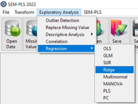
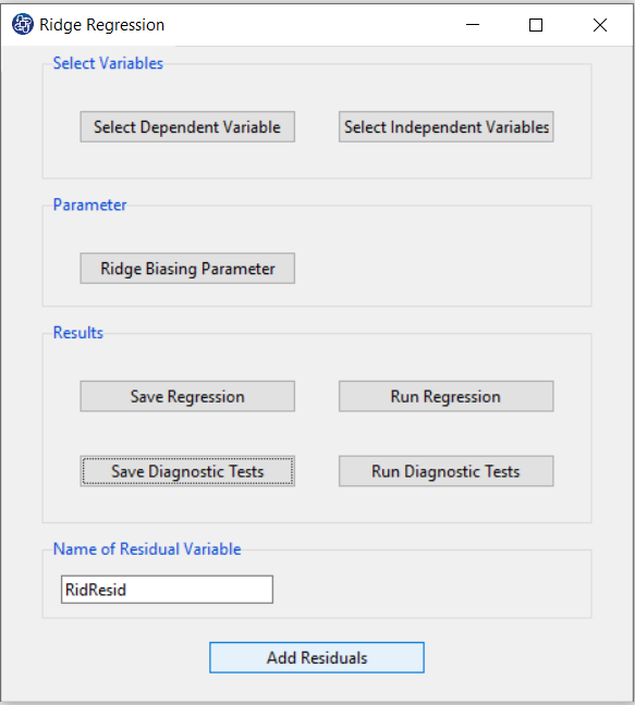
Path of Ridge Regression:

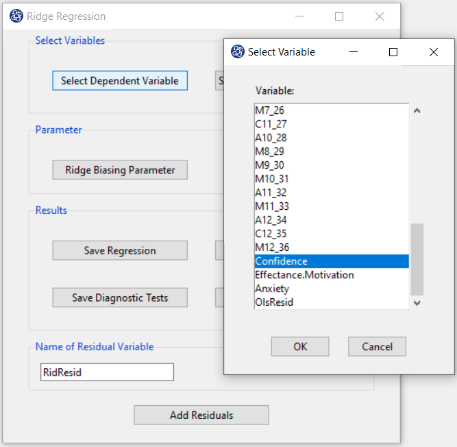
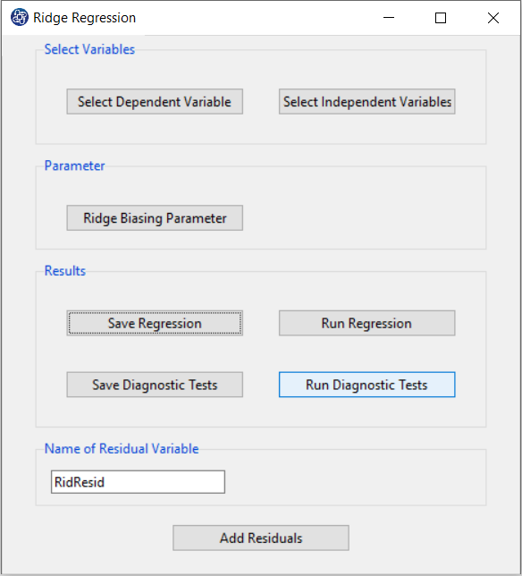
A. Select Dependent Variable:

You can select the dependent variable through this button. After opening the window, you can select it by selecting the desired variable.
For example, the variable Confidence is selected in this data.

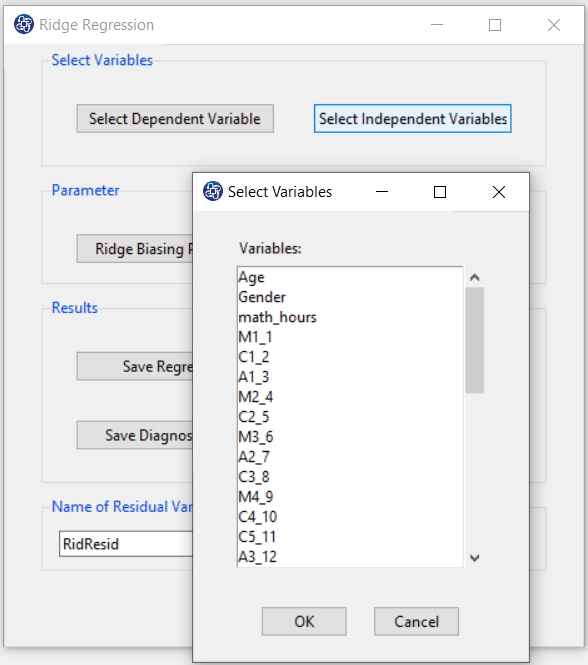
Select Independent Variables:

You can select the independent variables through this button. After the window opens, you can select them by selecting the desired variables.
For example, the variables Effectance Motivation and Anxiety are selected in this data.

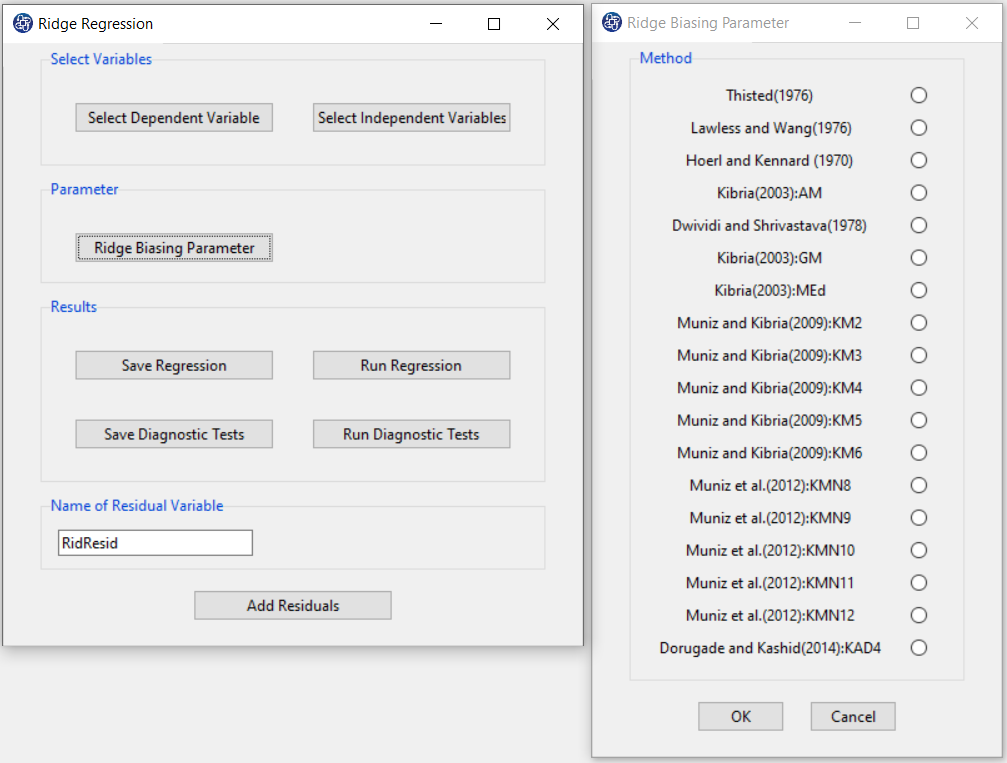
C. Ridge Biasing Parameter:

Table 1 lists various methods for the selection of biasing parameter k, proposed by different researchers.

Table1:Different available methods to estimate k

Reference	Biasing Parameter k
Thisted(1976)
Lawless and Wang (1976)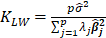
Hoerl and Kennard(1970a)
Kibria(2003)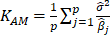
Dwividi and Shrivastava(1976)
Kibria (2003)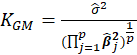
Kibria (2003)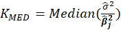
Muniz and Kibria (2009)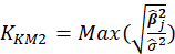
Muniz and Kibria (2009)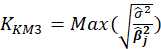
Muniz and Kibria (2009)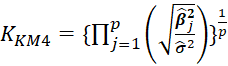
Muniz and Kibria (2009)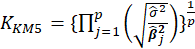
Muniz and Kibria (2009)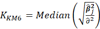
Muniz et al. (2012)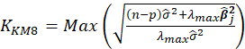
Muniz et al. (2012)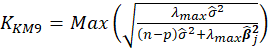
Muniz et al. (2012)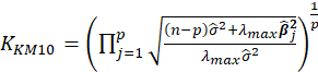
Muniz et al. (2012)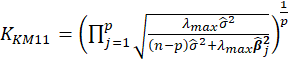
Muniz et al. (2012)
Dorugade(2014)
Note: s are eigenvalues of the correlation matrix

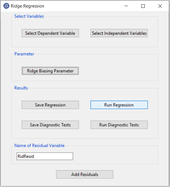
D. Run Regression:

You can see the results of the Ridge regression in the main window by clicking this button.
You can perform Ridge regression by the following path:
- Parameter Estimates
- Ridge Summary
- Collinearity Diagnostics

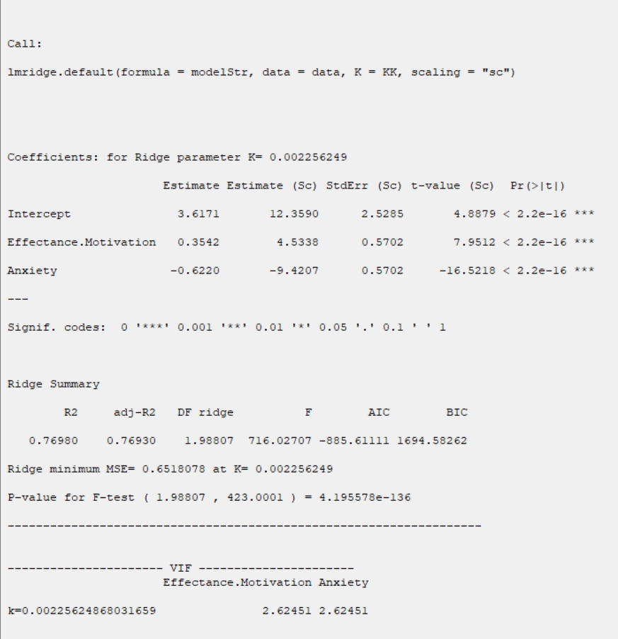
D1. Results:

In the Parameter Estimates table, estimation of coefficients and their significance are presented:

*Estimate:

Where k is Ridge Biasing Parameter.

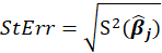
*StdErr:

is an estimate of the variance of given by the jth diagonal element of the matrix Also, k is Ridge Biasing Parameter. Thus,

*Estimate (SC) and StdErr(SC):

In this method, Estimation is based on the scaling method. The scaling method scales the predictors to correlation form, such that the correlation matrix has unit diagonal elements.

*t-value:

Halawa and El-Bassiouni (2000) presented to tackle the problem of testing 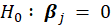by considering a non-exact t type test of the form


is an estimate of the variance of given by the jth diagonal element of the matrix . Also, k is Ridge Biasing Parameter.

*Pr(>|t|):

P-Value=Pr(|t|>t_n-p-1)

Ridge Summary:

In the Ridge Summary table, the evaluation criteria of regression model are presented.

These criteria include the following

*R2:

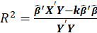
  Where, k is Ridge Biasing Parameter.

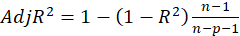
*adj-R2:

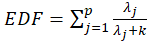
*DF ridge:

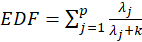
Where s are eigenvalues of the correlation matrix and k is Ridge Biasing Parameter.

*F:

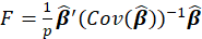
Where

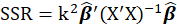
*AIC:

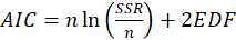
Where and s are eigenvalues of the correlation matrix and k is Ridge Biasing Parameter.Also,

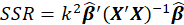
*BIC:

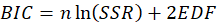
Where and s are eigenvalues of the correlation matrix and k is Ridge Biasing Parameter.Also,

P-Value for F-test:

we wish to test





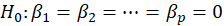
The P-value for this test is obtained from the following equation:

P-value=Pr(F> )
Where



k is Ridge Biasing Parameter

s are eigenvalues of the correlation matrix and k is Ridge Biasing Parameter.

MSE:

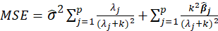
Where s are eigenvalues of the correlation matrix and k is Ridge Biasing Parameter.

*Collinearity Diagnostics:

In the Collinearity Diagnostics table, the results of multicollinearity in a set of multiple regression variables are given.

For each independent variable, the VIF index is calculated in two steps:

STEP1:

First, we run an ordinary least square regression that has x_i as a function of all the other explanatory variables in the first equation.

STEP2:

Then, calculate the VIF factor with the following equation:

Where is the coefficient of determination of the regression equation in step one. Also,

A rule of decision making is that if hen multicollinearity is high (a cutoff of 5 is also commonly used)

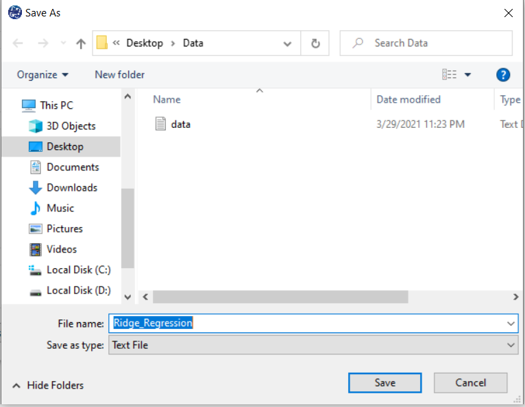
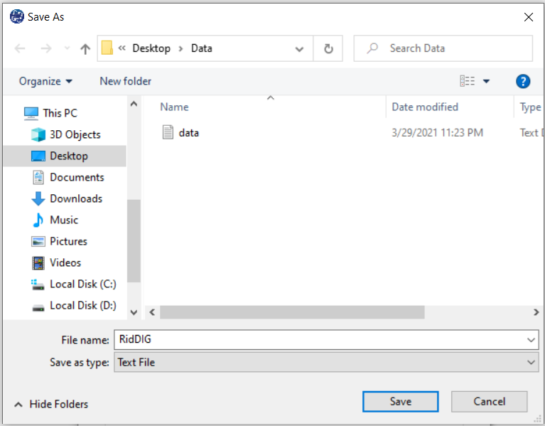
E. Save Regression:

By clicking this button, you can save the regression results. After opening the Save window, you can save the results in “text” or “Microsoft Word” format.

F. Run Diagnostic Tests:

In Ridge Regression, we shall make the following assumptions:

1-The residuals are independent of each other.

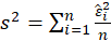
2- The residuals have a common variance

3- It is sometimes additionally assumed that the errors have the normal distribution. For example, if the residuals are normal, the correlation test can replace the independence test.

The following tests are provided to test these assumptions:

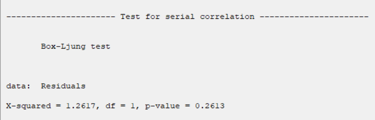
* Test for Serial Correlation:

-Box Ljung:

The test statistic is:
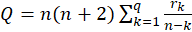
Where

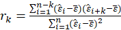
The sample autocorrelation at lag and is the number of lags being tested. Under , .

In this software, we give the results for q=1.

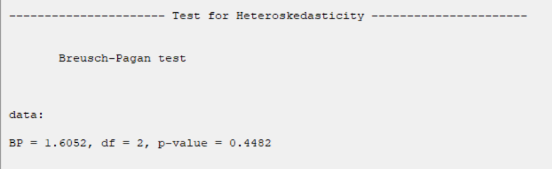
*Test for Heteroscedasticity:

-Breusch Pagan:

The test statistic is calculated in two steps:

STEP1:

Estimate the regression:

 Where  ,

STEP2:

Calculate the test statistic:

 Under  ,

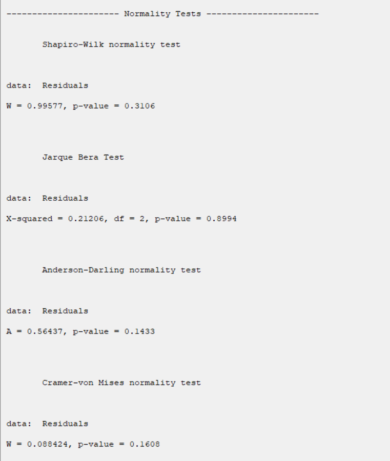
*Normality Tests:

-Shapiro Wilk:

The Shapiro-Wilk Test uses the test statistic

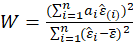
where the     values are given by:




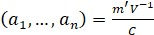
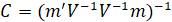
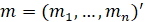is made of the expected values of the order statistics of independent and identically distributed random variables sampled from the standard normal distribution; finally, V is the covariance matrix of those normal order statistics. is compared against tabulated values of this statistic's distribution.

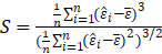
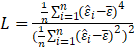
-Jarque Bera:

The test statistic is defined as

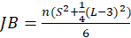
 Where 




 Under  , .

-Anderson Darling:

The test statistic is given by: .
where F(⋅) is the cumulative distribution of the normal distribution. The test statistic can then be compared against the critical values of the theoretical distribution.

-Cramer Von Mises:

The test statistic is given by:
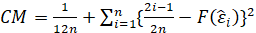
Where F(⋅) is the cumulative distribution of the normal distribution. The test statistic can then be compared against the critical values of the theoretical distribution.

G.1. Normality Tests:

The results show that in all tests, the P-value is greater than 0.05. Therefore, at 0.95 confidence level, the normality of the regression model residues is confirmed.

G.2. Test for Heteroscedasticity:

The results show that in all tests, the P-value is greater than 0.05. Therefore, 0.95 confidence level, the homogeneity of variance of residues is confirmed.

G.3. Test for Serial Correlation:

The results show that in all tests, the P-value is greater than 0.05. Therefore, at 0.95 confidence level, the independence of residues is confirmed.

H. Save Diagnostic Tests:

By clicking this button, you can save the diagnostic tests results. After opening the save results window, you can save the results in “text” or “Microsoft Word” format.

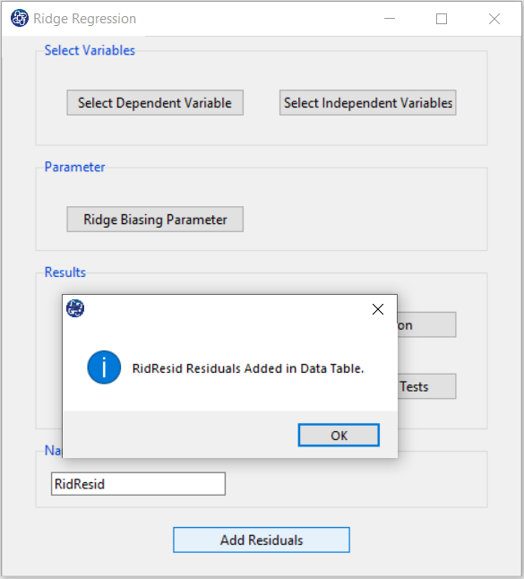
I. Add Residuals & Name of Residual Variable:

By clicking on this button, you can save the Residuals of the regression model with the desired name (Name of Residual Variable). The default software for the residual names is “RidgResid”.

I1. Add Residuals(verify message):

This message will appear if the residuals are saved successfully: “Name of Residual Variable Residuals added in Data Table.” For example, “RidResid Residuals added to the Data Table.”.