Example Variables(Open Data):
The Fennema-Sherman Mathematics Attitude Scales (FSMAS) are among the most popular instruments used in studies of
attitudes toward mathematics. FSMAS contains 36 items. Also, scales of FSMAS have Confidence, Effectance Motivation,
and Anxiety. The sample includes 425 teachers who answered all 36 items. In addition, other characteristics of teachers,
such as their age, are included in the data.
You can select your data as follows:
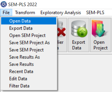
1-File
2-Open data
(See Open Data)
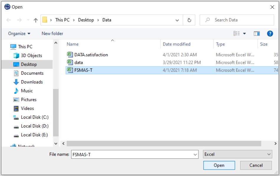
The data is stored under the name FSMAS-T(You can download this data from
here ).
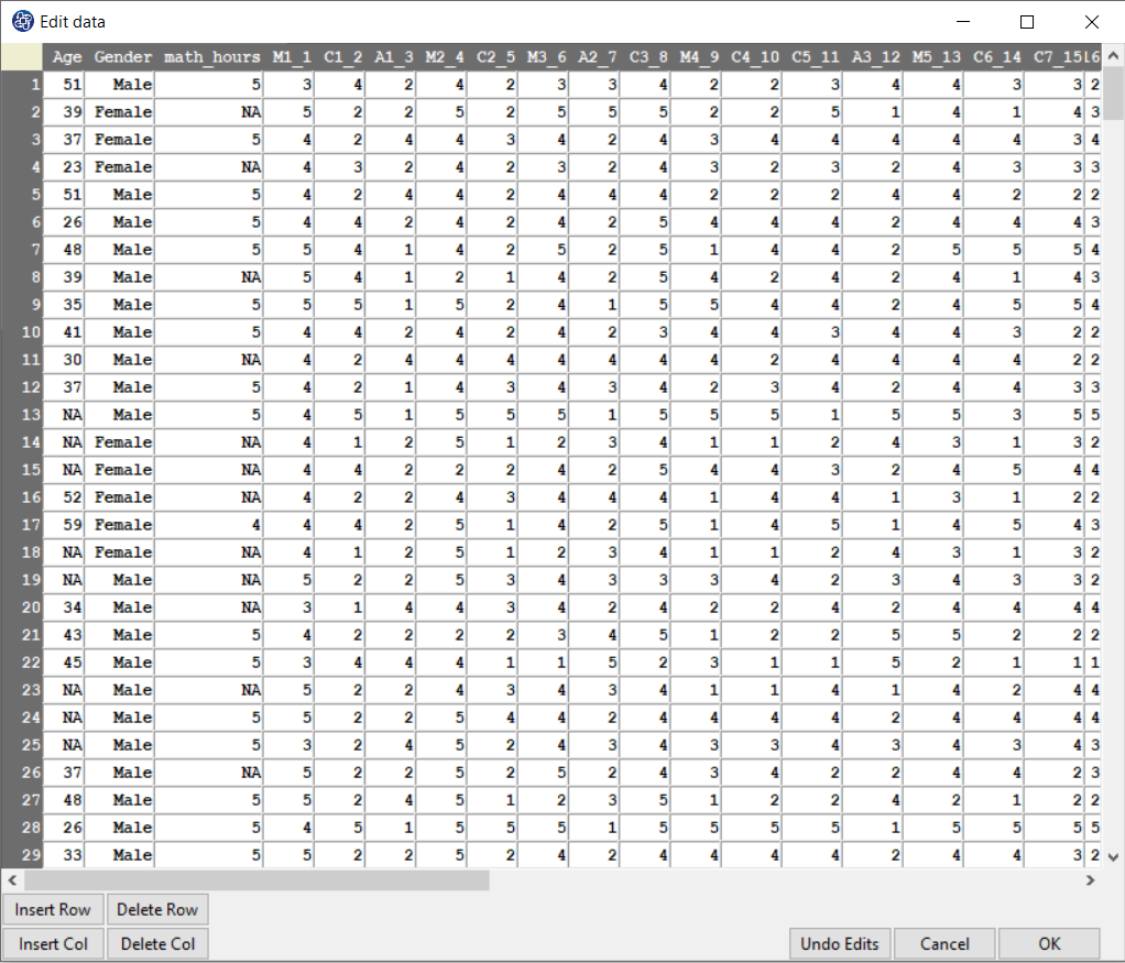
You can edit the imported data via the following path:
1-File
2-Edit Data
(See Edit Data)
Example Variables(Compute Variable):
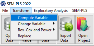
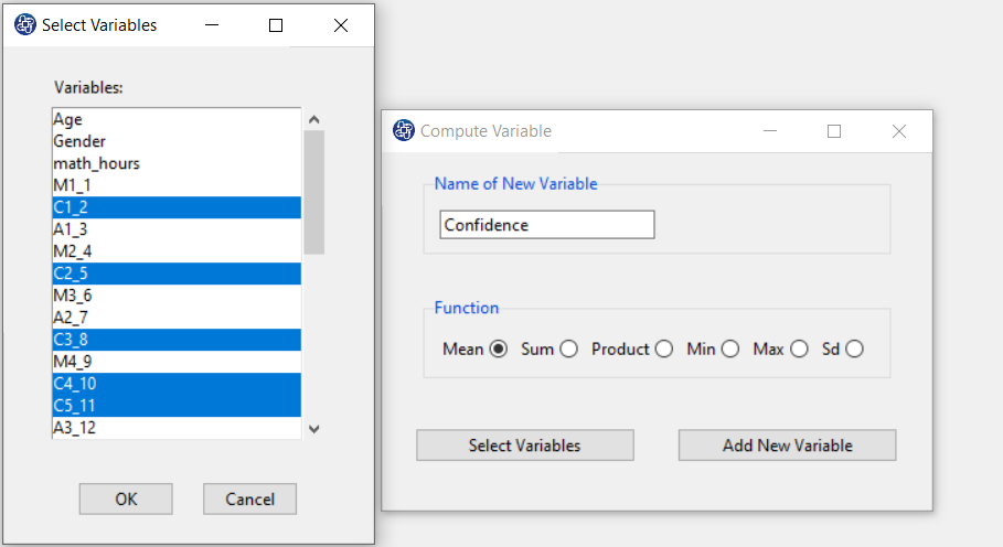
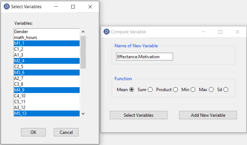
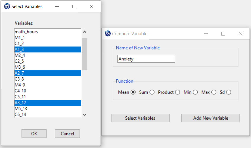
The three variables of Confidence, Effectance Motivation, and Anxiety can be calculated through the following path:
1-Transform
2-Compute Variable
Items starting with the letters C, M, and A are related to the variables Confidence, Effectance Motivation, and Anxiety, respectively.
(See Compute Variable)
Introduction to Regression
Suppose each observation i includes a scalar dependent variable yi and column vector of values of p independent
variables xi1 , xi2 , xi3 ,…, xip .
A linear regression is a linear function of independent variables:

This model can also be written in matrix notation as
Where y and
 are
are
 vectors of the values of the response variable and the errors for the various observations, and
 is an
is an
 matrix.
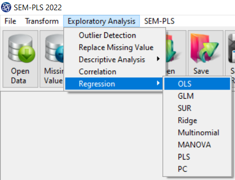
Path of OLS Regression
You can perform OLS regression by the following path:
1-Exploratory Analysis
2- Regression
3-OLS
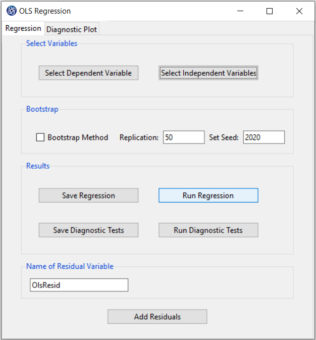
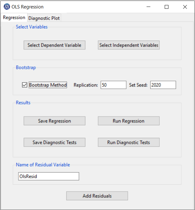
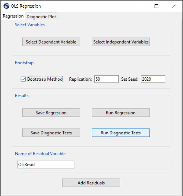
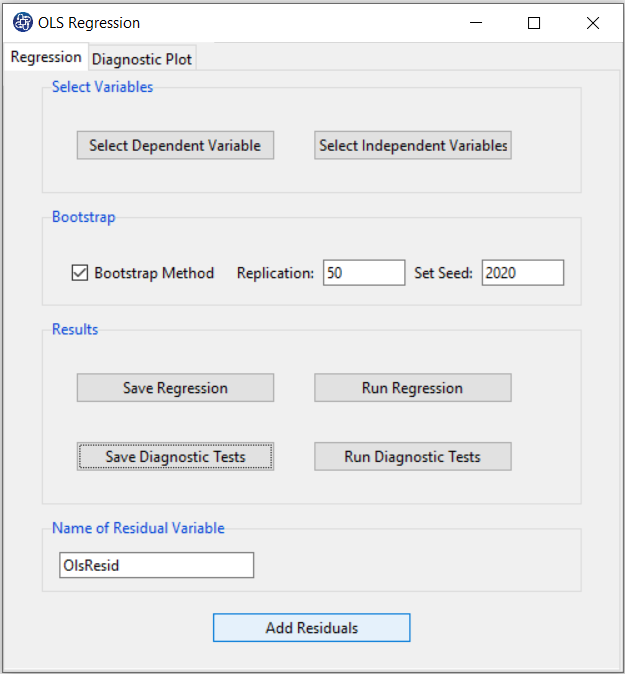
A. OLS Regression window:
OLS Regression window includes two tabs, Regression and Diagnostic Plot.
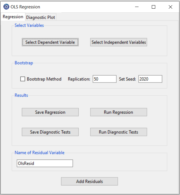
B. Regression
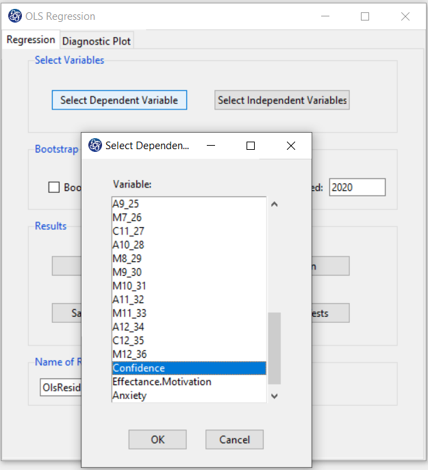
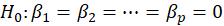
B1. Select Dependent Variable:
You can select the dependent variable through this button. After opening the window,
you can select it by selecting the desired variable.
For example, the variable Confidence is selected in this data.
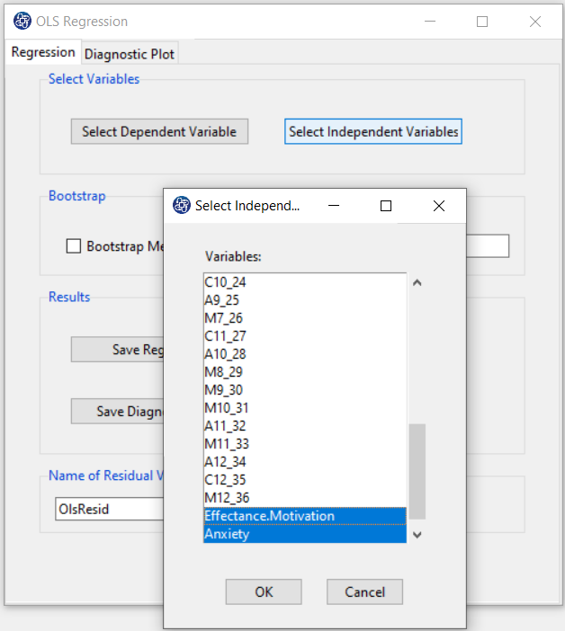
B2. Select Independent Variables:
You can select the independent variables through this button. After the window opens,
you can select them by selecting the desired variables.
For example, the variables Effectance Motivation and Anxiety are selected in this data.
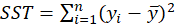
B3. Run Regression:
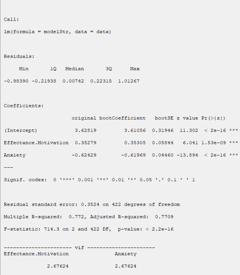
You can see the results of the OLS regression in the results panel by clicking this button.
Results include the following:
-Model Summary
-ANOVA
-Parameter Estimates
-Collinearity Diagnostics
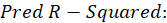
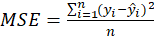
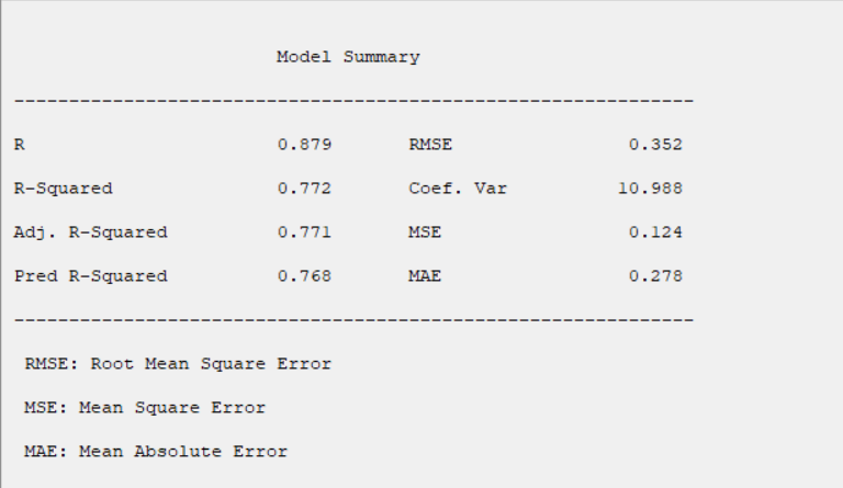
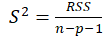
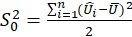
B3.1. Result( Model Summary):
In the Model Summary table, the evaluation criteria of the regression model are presented.
These criteria include the following:
*

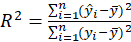
*R:

*
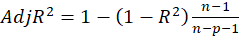
*
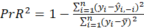
Where
 is prediction of
 after removing this variable from the data.
*MSE:
*RMSE:
*MAE:
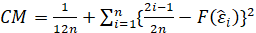
*CV:
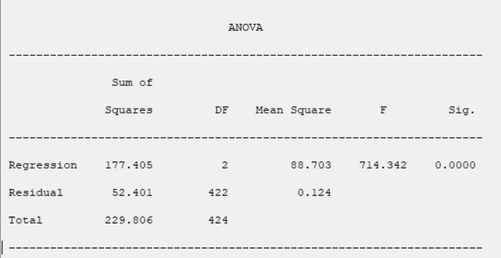
B3.2. Result(ANOVA):
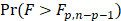
In the ANOVA table, The results of the model significance test are given.
we wish to test

we define the following terminology:
The usual way of setting out this test is to use the following:
| Sum of Squares | DF | Mean Square | F | Sig. | |
|---|---|---|---|---|---|
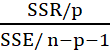
| Regression | SSR | P | SSR/p |
|
|
| Residual | SSE | n-p-1 | SSE/ n-p-1 | ||
| Total | SST | n-1 |
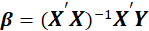
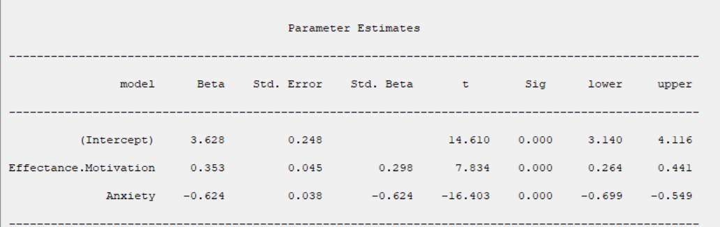
A4.3. In the Parameter Estimates table, the results of estimating the coefficients of the independent variables are given.
The coefficients presented in this table are obtained from the following relationships:
*Beta:
*Std. Error:
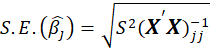
Where
 .
.
*Std. Beta:

Where
 and
and
 are standard deviation of
 and
and
 respectively.
*t:

*Sig:
P-Value=Pr(|t|>tn-p-1)
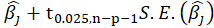
*95% Confidence Interval for
 :
:
lower:
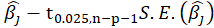
upper:
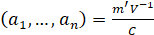
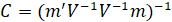
B3.3. Result(Collinearity Diagnostics):
In the Collinearity Diagnostics table, the results of multicollinearity in a set of multiple regression variables are given.
For each independent variable, the VIF index is calculated in two steps:
STEP1:
First, we run an ordinary least square regression that has xi as a function of all the other explanatory variables in the first equation.
STEP2:
Then, calculate the VIF factor with the following equation:

Where
 is the coefficient of determination of the regression equation in step one. Also,
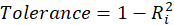 .
.
A rule of decision making is that if
 then multicollinearity is high (a cutoff of 5 is also commonly used)
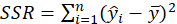
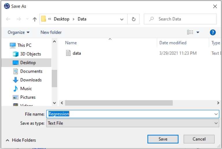
B4. Save Regression:
By clicking this button, you can save the regression results. After opening the save results window, you can save the results in “text” or “Microsoft Word” format.
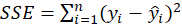
B5: Bootstrap:
This panel includes the following methods:
Assume that we want to fit a regression model with dependent variable y and predictors
x1, x2,..., xp. We have a sample of n observations zi =
(yi,xi1, xi2,...,xip)
where i= 1,...,n. In random x resampling, we simply select B( Replication)
bootstrap samples of the zi, fitting the model and saving the
 and
and
 and from each bootstrap sample. The statistic t is normally distributed (which is often approximately
the case for statistics in sufficiently large Replication). If
and from each bootstrap sample. The statistic t is normally distributed (which is often approximately
the case for statistics in sufficiently large Replication). If
 is the corresponding estimate for the ith bootstrap replication and
 is the mean of the
s
,
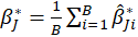
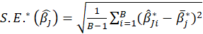
then the bootstrap estimation and the bootstrap standard error are
is the mean of the
s
,
then the bootstrap estimation and the bootstrap standard error are
Thus

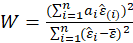
*Bootstrap Method:
Enabling this option means performing regression using the bootstrap method with the following parameters:
*Replication: Number of Replication(B in equations)
*Set Seed: It is an arbitrary number that will keep the Bootstrap results fixed by holding it fixed.
B5.2. Result(Bootstrap):
Running regression with the Bootstrap option enabled provides the following results:
Original:
bootCoefficient:

bootSE:

z value: z
B6. Run Diagnostic Tests:
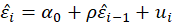
In OLS Regression, we shall make the following assumptions:
1-The residuals are independent of each other.
2- The residuals have a common variance
 .
.
3- It is sometimes additionally assumed that the errors have the normal distribution.
For example, if the residuals are normal, the correlation test can replace the independence test.
The following tests are provided to test these assumptions:
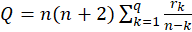
* Test for Serial Correlation:
-Breusch Godfrey:
If the following auxiliary regression model is fitted

and if the usual
 statistic is calculated for this model, then the following asymptotic approximation can be used for the distribution of the test statistic
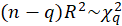
When
 In this software, we give the results for q=1.
-Durbin Watson:
If
the Durbin-Watson statistic states that null hypothesis:

the Durbin Watson statistic is
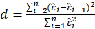
Exact critical values for the distribution of d under the null hypothesis of no serial correlation
can be calculated. Under
 , d is distributed as
 .
.
Where
 s
are independent standard normal random variables; and the
s
are the nonzero eigenvalues of
s
are independent standard normal random variables; and the
s
are the nonzero eigenvalues of
Where
 .
.
-Box Ljung:
The test statistic is:
Where
 .
.
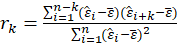
The sample autocorrelation at lag
 and
and
 is the number of lags being tested. Under
,
is the number of lags being tested. Under
,
 .
.
In this software, we give the results for q=1.
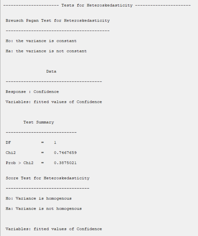
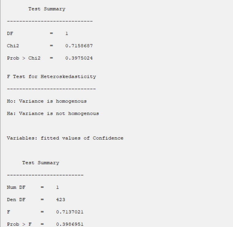
*Test for Heteroscedasticity:
-Breusch Pagan:
Test statistic is calculated in two steps:
STEP1:
Estimate the regression:
Where
 ,
,
STEP2:
Calculate the
 test statistic:
 Under
,
Under
,
 .
.
-Score:
Test statistic is calculated in two steps:
STEP1:
Estimate the regression:
Where
,
STEP2:
Calculate the
test statistic:
Under
,
.
-F:
Test statistic is calculated in two steps:
STEP1:
Estimate the regression:
Where
,
STEP2:
Calculate the
 Under
,
Under
,
 .
.
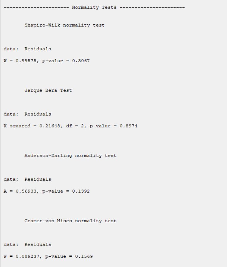
*Normality Tests:
-Shapiro Wilk:
The Shapiro-Wilk Test uses the test statistic
where the
 values are given by:
 is made of the expected values of the order statistics of independent and identically distributed random variables sampled from the standard normal distribution;
finally, V is the covariance matrix of those normal order statistics.
is made of the expected values of the order statistics of independent and identically distributed random variables sampled from the standard normal distribution;
finally, V is the covariance matrix of those normal order statistics.
 is compared against tabulated values of this statistic's distribution.
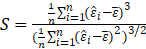
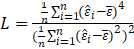
-Jarque Bera:
The test statistic is defined as
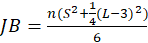
Where
Under
,
 .
.
-Anderson Darling:
The test statistic is given by:

where F(⋅) is the cumulative distribution of the normal distribution.
The test statistic can then be compared against the critical values of the theoretical distribution.
-Cramer Von Mises:
The test statistic is given by:
where F(⋅) is the cumulative distribution of the normal distribution. The test statistic can then be compared against
the critical values of the theoretical distribution.
B6.1. Normality Tests:
The results show that in all tests, the P-value is greater than 0.05. Therefore, at 0.95 confidence level, the normality of the regression model residues is confirmed.
B6.2. Test for Heteroscedasticity:
The results show that in all tests, the P-value is greater than 0.05. Therefore, 0.95 confidence level, the homogeneity of variance of residues is confirmed.
B6.3. Test for Serial Correlation:
The results show that in all tests, the P-value is greater than 0.05. Therefore, at 0.95 confidence level, the independence of residues is confirmed.
B7. Save Diagnostic Tests:
By clicking this button, you can save the results of the diagnostic tests. After opening the save results window, you can save the results in “text” or “Microsoft Word” format.
B8. Add Residuals & Name of Residual Variable:
By clicking on this button, you can save the residuals of the regression model with the desired name(Name of Residual Variable). The default software for the residual names is “OlsResid”.
B9. Add Residuals(verify message):
This message will appear if the balances are saved successfully:
“Name of Residual Variable Residuals added in Data Table.”
For example,
“OlsResid Residuals added in Data Table.”.

C. Diagnostic Plot:
In the Diagnostic Plot tab, diagnostic plots help you to better identify the behavior of the model residues.
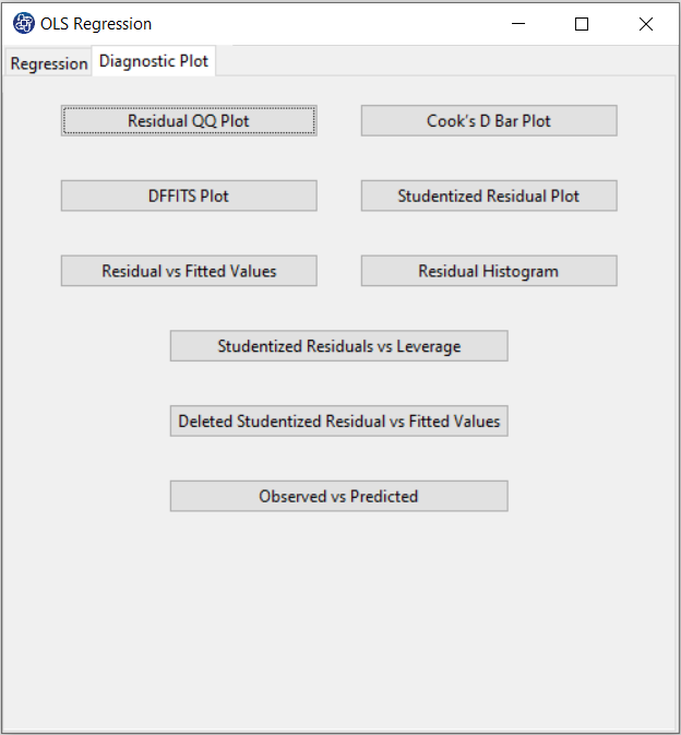
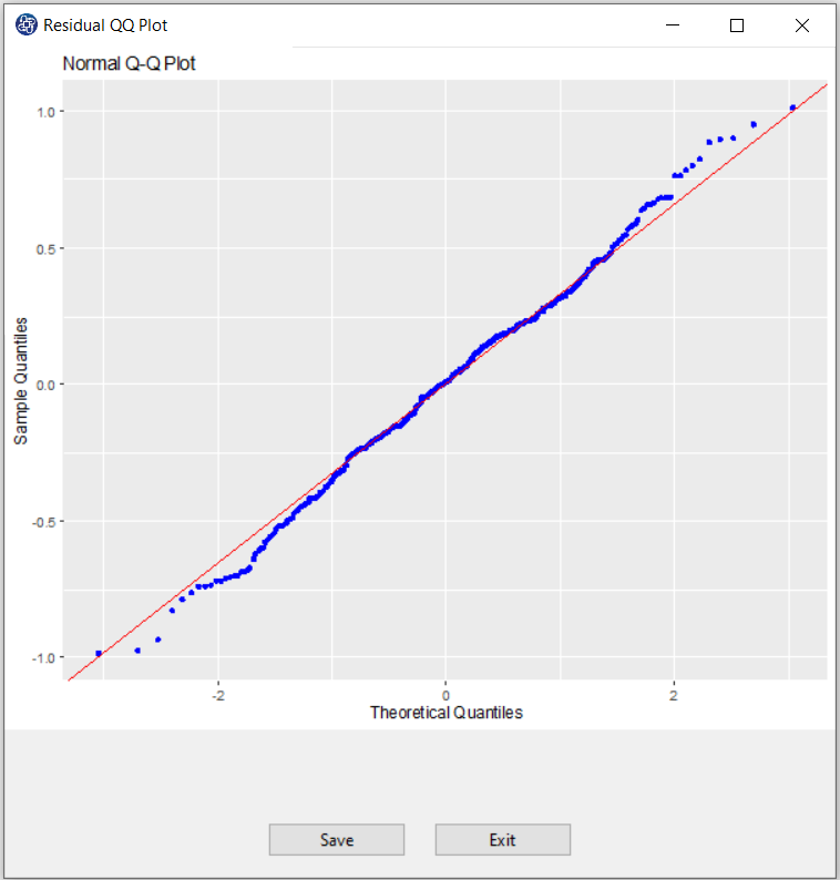
C1. Normal QQ Plot:
If the residuals follow a normal distribution with mean μ and variance σ^2, then a plot of the theoretical percentiles of the normal distribution(Theoretical Quantiles) versus the observed sample percentiles of the residuals(Sample Quantiles) should be approximately linear. If a Normal QQ Plot is approximately linear, we assume that the error terms are normally distributed.
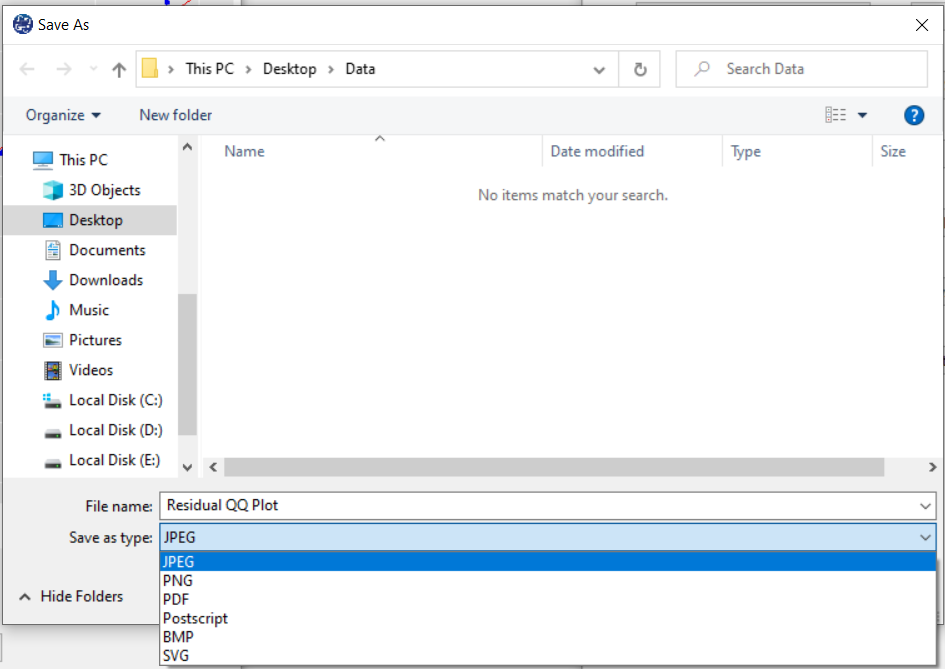
C2. Save plot:
You can save the plot by clicking the Save button in one of the following formats:
-JPEG
-PNG
-PDF
-Postscript
-BMP
-SVG
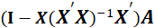
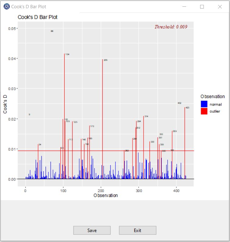
C3. Cook’s D Bar Plot:
Cook’s distance is obtained in three steps:
Delete observations one at a time
Refit the regression model on remaining n-1 observations
Examine how much all of the fitted values change when the ith observation is deleted.
Cook’s distance is obtained from the following relation:
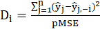
Where
 is the fitted dependent value when excluding
 ,
,
 .
.
Cook’s D Bar Plot to detect observations that strongly influence fitted values of the mode.
It is used to identify influential data points.
It depends on both the residual and leverage i.e it takes it account both the x value and y value of the observation.
Threshold of plot is
 .
.
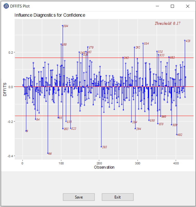
C4. DFFITS Plot:
DFFITS is the scaled difference between the ith fitted value obtained from the full data and the ith
fitted value obtained by deleting the ith observation.
DFFITS is obtained in three steps:
Delete observations one at a time.
Refit the regression model on remaining n-1 observations
Examine how much all of the fitted values change when the ith observation is deleted.
DFFITS is obtained from the following relation:
Where
 and
and
 are the fitted dependent value and
 when excluding
. Also,
when excluding
. Also,
 ,
,
 .
.
An observation is deemed influential if the absolute value of its DFFITS value is greater than:

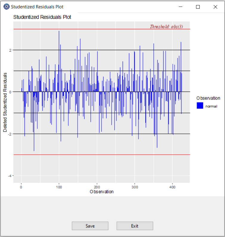
C5. Studentized residuals Plot:
A studentized deleted (or externally studentized) residual is:
Where
 are the mean square error when excluding
. Also,
are the mean square error when excluding
. Also,
 ,
,
 .
.
Studentized deleted residuals is the deleted residual divided by its estimated standard deviation.
Studentized residuals are going to be more effective for detecting outlying y observations than standardized
residuals. If an observation has an externally studentized residual that is larger than 3 (in absolute value)
we can call it an outlier.
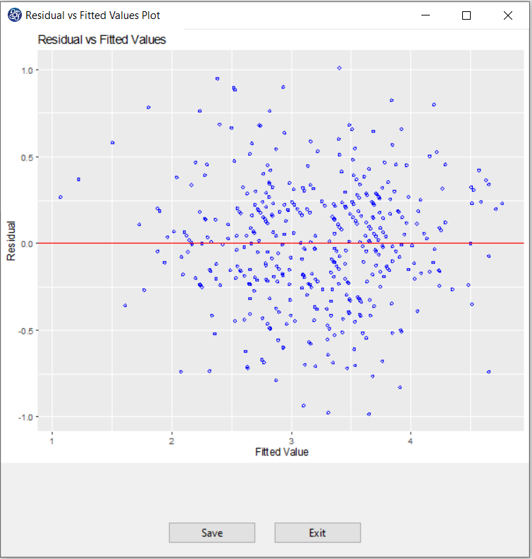
C6. Residual vs Fitted Values Plot:
When conducting a residual analysis, a "residuals versus fits plot" is the most frequently created plot. It is a scatter plot of residuals on the y axis and fitted values (estimated responses) on the x axis. The plot is used to detect non-linearity, unequal error variances, and outliers.
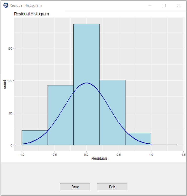
C7. Residual Histogram:
The histogram of the residual can be used to check whether the residuals is normally distributed. A symmetric bell-shaped histogram which is evenly distributed around zero indicates that the normality assumption is likely to be true.
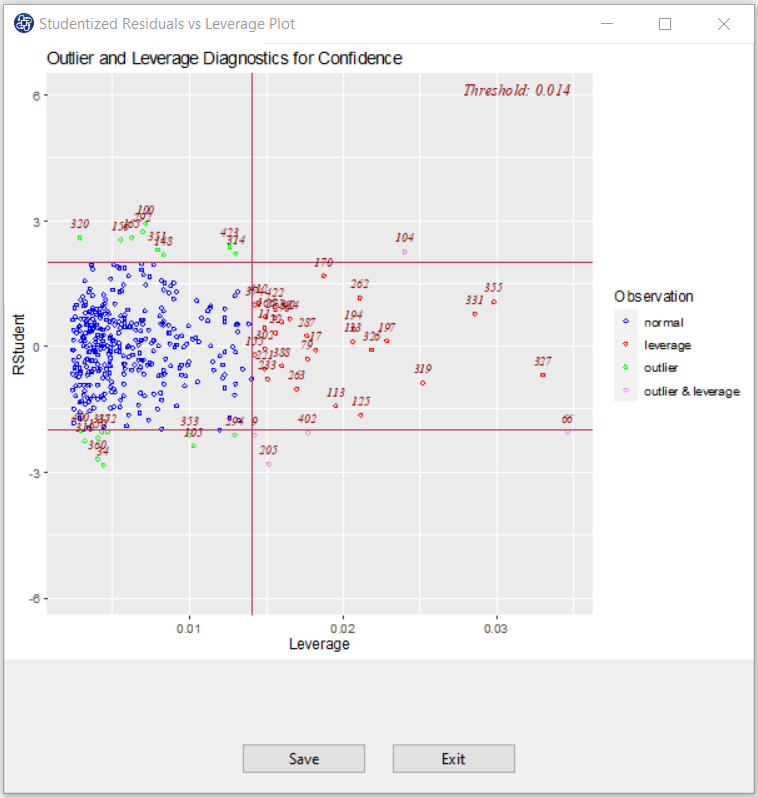
C8. Studentized residuals vs Leverage Plot:
This plot shows that how the spread of standardized residuals changes as the leverage, or sensitivity of the fitted
 to a change in
, increases.
to a change in
, increases.
This can also be used to detect heteroskedasticity and non-linearity.
The spread of standardized residuals shouldn’t change as a function of leverage.
Points with high leverage may be influential. Threshold of plot is
 . Also, the absolute value of an observation is deemed influential if it is greater than 2.
C9. Deleted Studentized Residuals vs Fitted Values Plot:
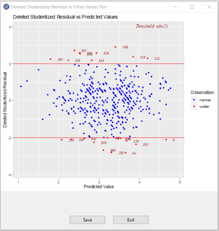
It is a scatter plot of residuals on the y axis and the predictor values on the x axis. The interpretation of this plot is identical to that for a "Residual vs Fitted Values Plot" That is, a well-behaved plot will bounce randomly and form a roughly horizontal band around the residual = 0 line. And, no data points will stand out from the basic random pattern of the other residuals. An observation is deemed influential if its absolute is greater than 2.
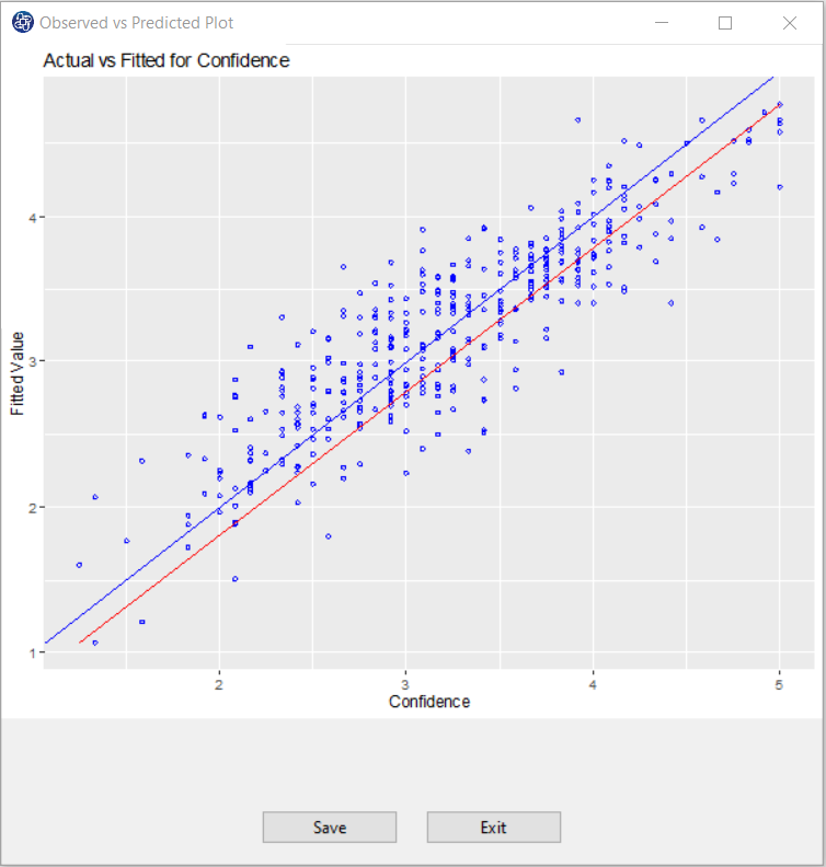
C10. Observed vs Predicted Plot:
A predicted against actual plot shows the effect of the model and compares it against the null model. For a good fit, the points should be close to the fitted line, with narrow confidence bands. Points on the left or right of the plot, furthest from the mean, have the most leverage and effectively try to pull the fitted line toward the point. Points that are vertically distant from the line represent possible outliers. Both types of points can adversely affect the fit.