Example Variables(Open Data):
The Fennema-Sherman Mathematics Attitude Scales (FSMAS) are among the most popular instruments used in studies of
attitudes toward mathematics. FSMAS contains 36 items. Also, scales of FSMAS have Confidence, Effectance Motivation,
and Anxiety. The sample includes 425 teachers who answered all 36 items. In addition, other characteristics of teachers,
such as their age, are included in the data.
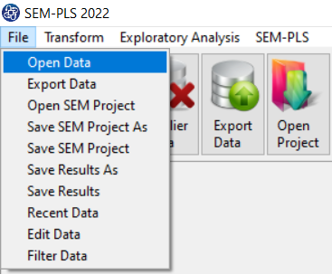
You can select your data as follows:
1-File
2-Open data
(See Open Data)
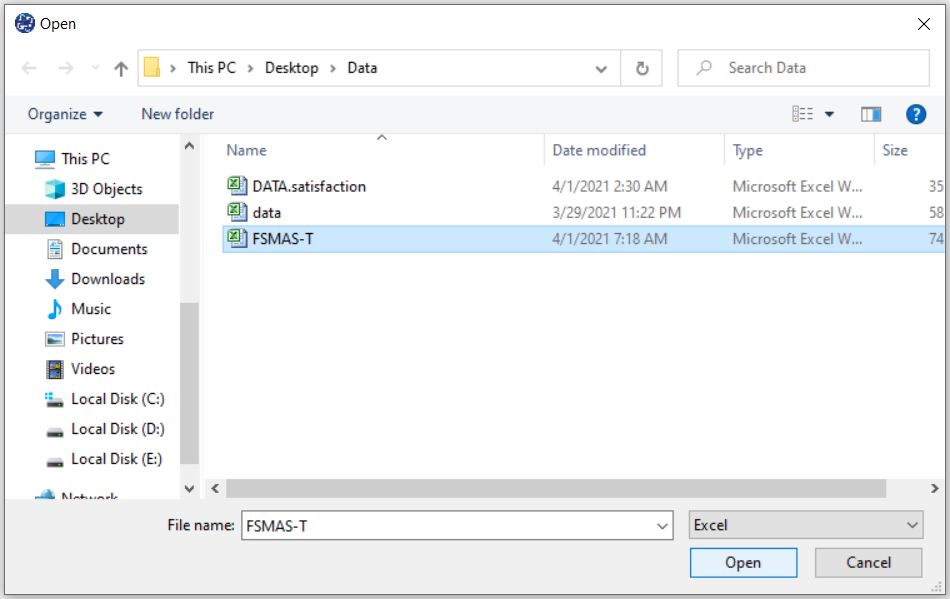
The data is stored under the name FSMAS-T(You can download this data from
here ).
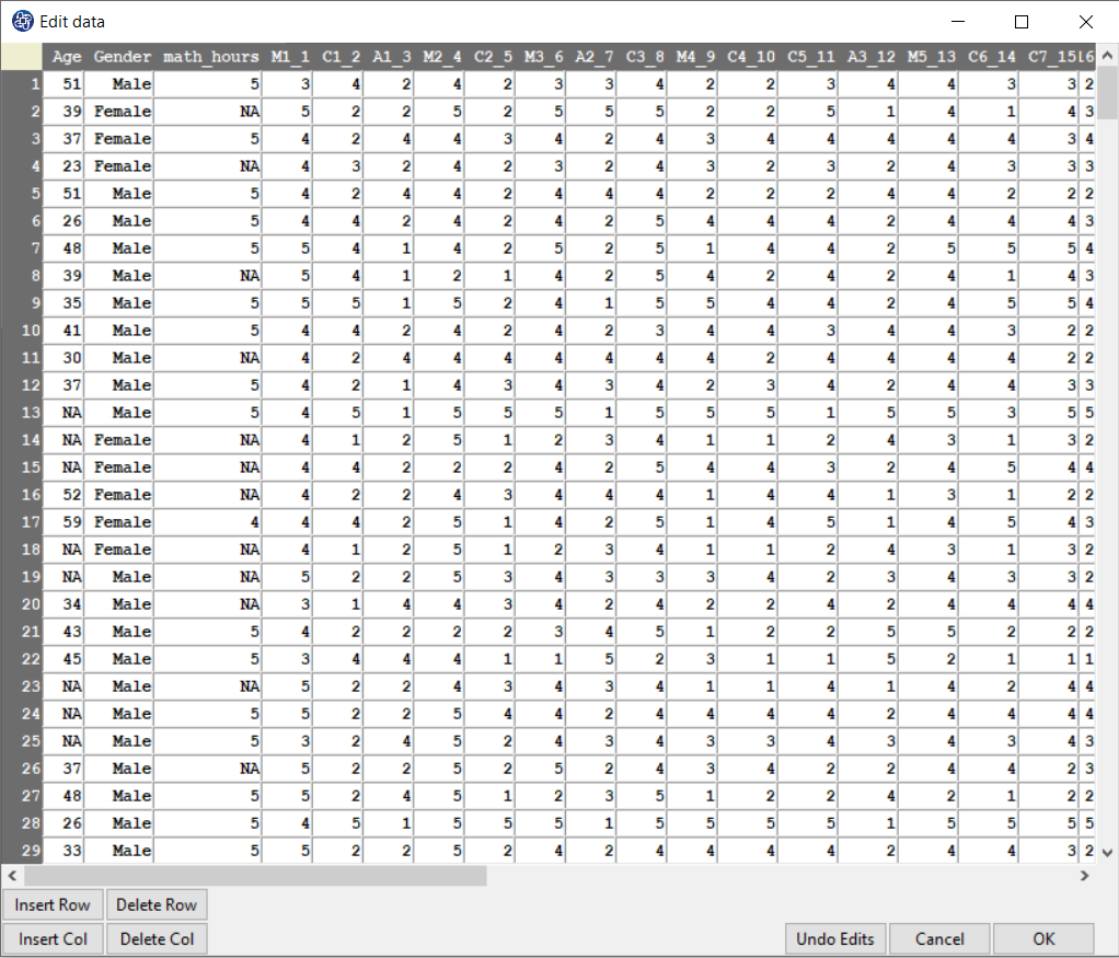
You can edit the imported data via the following path:
1-File
2-Edit Data
(See Edit Data)
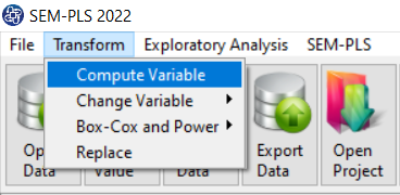
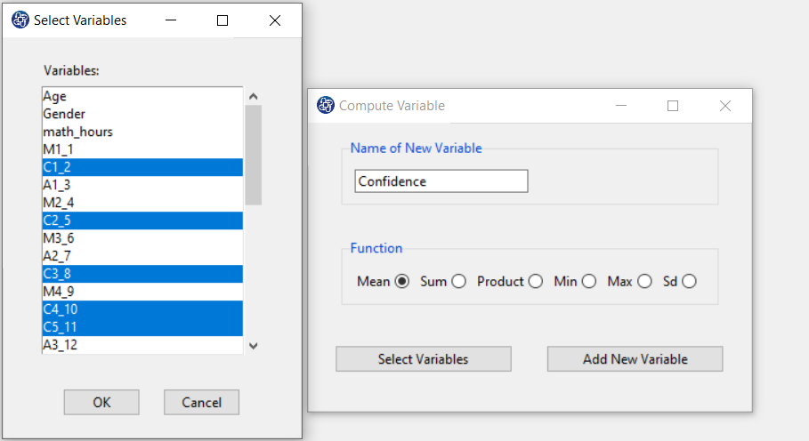
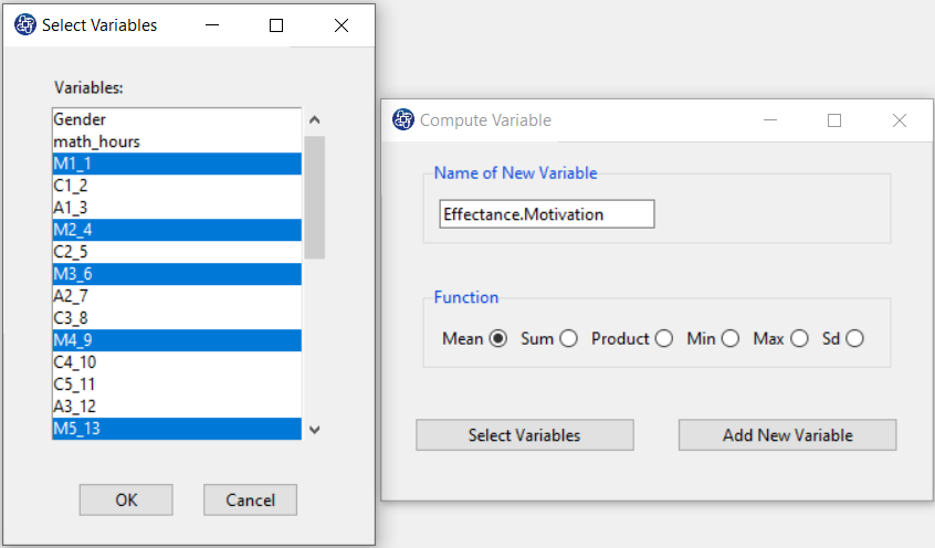
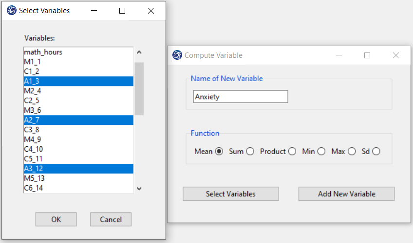
Example Variables(Compute Variable):
The three variables of Confidence, Effectance Motivation, and Anxiety can be calculated through the following path:
1-Transform
2-Compute Variable
Items starting with the letters C, M, and A are related to the variables Confidence, Effectance Motivation, and Anxiety, respectively.
(See Compute Variable)
Introduction to Partial Least Squares (PLS) Regression
The multiple linear regression can be written in matrix notation as
Where y and
 are
are
 vectors of the values of the response variable and the errors for the various observations, and
 is a
is a
 matrix.
In the multiple linear regression, the least-squares solution for
 is given by
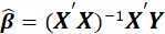 .
.
The problem often is that
 is singular, either because the number of variables (columns) in
 exceeds the number of objects (rows), or because of collinearities.
PLS Regression circumvent this by decomposing X into orthogonal scores
 and loadings


In this method, the components, called Latent Variables (LVs) in this context, are obtained iteratively.
One starts with the SVD(singular value decomposition) of the cross product matrix
 , thereby including information on variation in both
 and
and
 , and on the correlation between them. The first left and right singular vectors,
 and
and
 , are used as weight vectors for
 and
and
 , respectively, to obtain scores
 and
and
 :
:
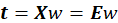
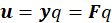
Where
 and
and
 are initialised as
and
, respectively. The
scores
are initialised as
and
, respectively. The
scores
 are often normalised:

The
scores
 are not actually necessary in the regression but are often saved for interpretation purposes. Next,
and
loadings are obtained by regressing against the same vector
:
are not actually necessary in the regression but are often saved for interpretation purposes. Next,
and
loadings are obtained by regressing against the same vector
:


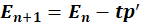
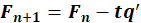
Finally, the data matrices are deflated: the information related to this latent variable, in the form of the outer products
 and
and
 , is subtracted from the (current) data matrices
and
.
, is subtracted from the (current) data matrices
and
.
The estimation of the next component can then start from the SVD of the cross-product matrix
 . After every iteration, vectors
,
,
. After every iteration, vectors
,
,
 and
are saved as columns in matrices
and
are saved as columns in matrices
 ,
,
 ,
,
 and
and
 , respectively. One complication is that columns of matrix
can not be compared directly: they are derived from successively deflated matrices
and
.
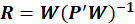
It has been shown that an alternative way to represent the weights, in such a way that all columns
relate to the original
matrix, is given by
, respectively. One complication is that columns of matrix
can not be compared directly: they are derived from successively deflated matrices
and
.
It has been shown that an alternative way to represent the weights, in such a way that all columns
relate to the original
matrix, is given by
Now, instead of regressing
on
,
we use scores
to calculate the regression coefficients, and later convert these back to the realm of the original
variables by pre-multiplying with matrix
 (since
 ):
):

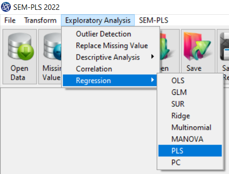
Path of PLS Regression:
You can perform PLS regression by the following path:
1-Exploratory Analysis
2- Regression
3-PLS
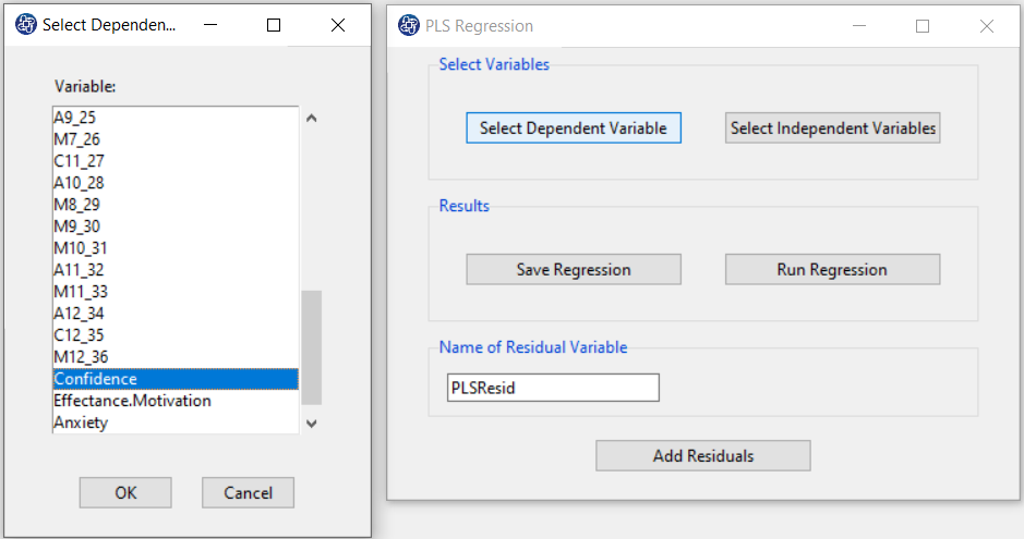
A. PLS Regression window:
After opening the PLS Regression window, you can start the model analysis process.
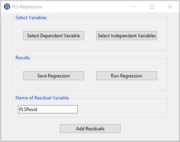
B. Select Dependent Variable:
You can select the dependent variable through this button. After opening the window,
you can choose it by selecting the desired variable.
For example, the variable Confidence is selected in this data.
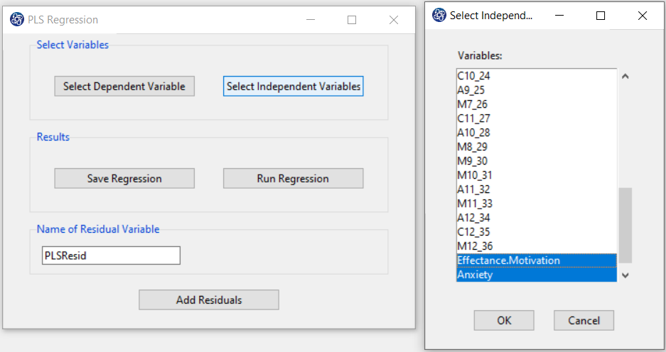
C. Select Independent Variables:
You can select the independent variables through this button. After the window opens,
you can select them by selecting the desired variables.
For example, the variables Effectance Motivation and Anxiety are selected in this data.
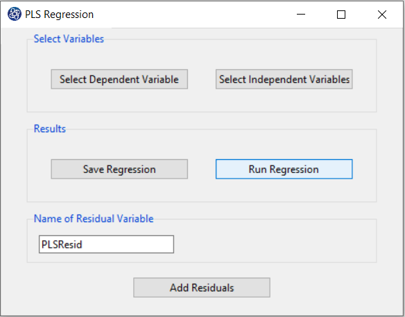
D. Run Regression:
You can see the results of the PLS regression in the main window by clicking this button.
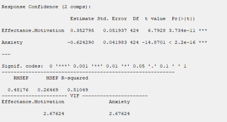
Results include the following:
-Parameter Estimates
-Model Summary
-Collinearity Diagnostics
E. Results:
Parameters are estimated based on the jack-knife method.
At first, all
and
variables are regarded as active. Then the following process was iterated automatically until each apparently useless
 and
variable had been detected as non-significant and made passive. The full leave-one-product-out cross-validation was
applied for the remaining active
and
variables, and the optimal rank
was determined. The approximate uncertainty variance of the PC regression coefficients
and
variable had been detected as non-significant and made passive. The full leave-one-product-out cross-validation was
applied for the remaining active
and
variables, and the optimal rank
was determined. The approximate uncertainty variance of the PC regression coefficients
 was then estimated by jack-knifing:
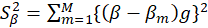
Where
 estimated uncertainty variance of

 the regression coefficient at the cross-validated rank
using all the
the regression coefficient at the cross-validated rank
using all the
 objects
 the regression coefficient at the rank
using all objects except the object left out in cross-validation segment
the regression coefficient at the rank
using all objects except the object left out in cross-validation segment


As a rough significance test a t-test (n degrees of freedom) was performed for each element in
relative to the square root of its estimated uncertainty variance
, and the optimum significance level was noted for each
variable and for each
variable.
*

*MSEP:
*RMSEP:
* Collinearity Diagnostics
In the Collinearity Diagnostics table, the results of multicollinearity in a set of multiple regression variables are given.
For each independent variable, the VIF index is calculated in two steps:
STEP1:
First, we run an ordinary least square regression that has xi as a function of all the other explanatory variables in the first equation.
STEP2:
Then, calculate the VIF factor with the following equation:
 Where
Where
 is the coefficient of determination of the regression equation in step one. Also,
A rule of decision making is that if
 then multicollinearity is high (a cutoff of 5 is also commonly used)
F. Save Regression:
By clicking this button, you can save the regression results. After opening the save results window, you can save the results in “text” or “Microsoft Word” format.
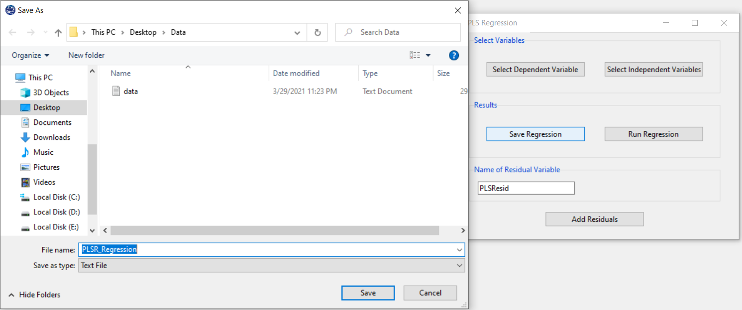
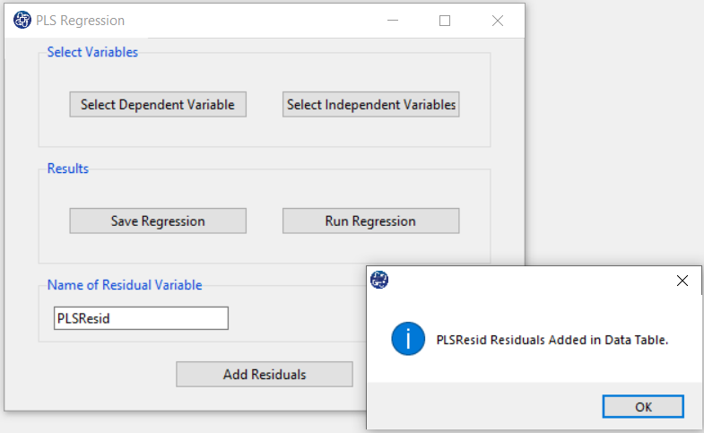
G. Add Residuals & Name of Residual Variable:
By clicking on this button, you can save the residuals of the regression model with the desired
name(Name of Residual Variable). The default software for the residual names is “PLSResid”.
This message will appear if the residuals are saved successfully:
“Name of Residual Variable Residuals added in Data Table.”
For example,
“PLSResid Residuals added in Data Table.”.